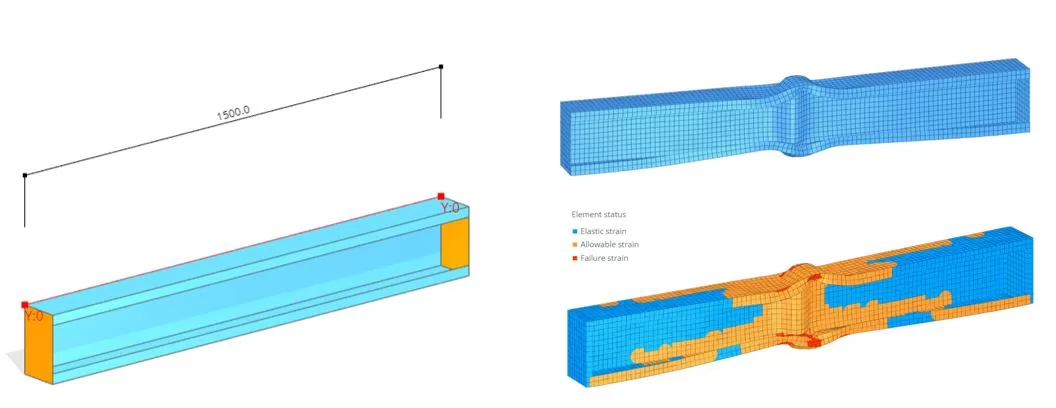
In this example, we will demonstrate how to analyze a member made from a thin steel plate profile. The profile has the channel section with a plate thickness of 1.5 mm and a length of 1500 mm. Diaphragms, with a thickness of 20 mm, are attached to both ends of the member. Boundary conditions are applied at the member’s ends: the left side is rolled while the opposite end is pinned. The material properties for the parts are defined with a yield strength (fy) of 355 MPa. The member is subject to an axial compressive force of 1000 kN.
To see this analysis in action and gain a better understanding, watch the quick video demonstration provided below:
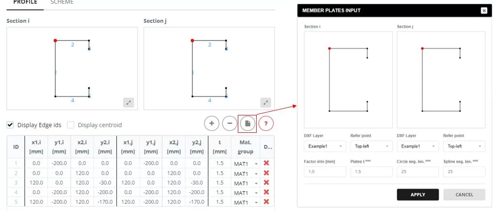
Step 1. Model Parts
Go to the ‘Main Parts’ menu and select the ‘PROFILE’ tab. Input the edges for both the starting (i) and ending (j) sections. To input the sections’ geometry, you can import a DXF file stored locally on your PC. The dxf file can be received from here
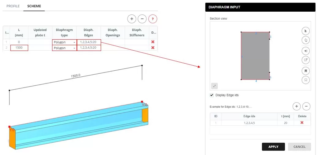
Go to the ‘SCHEME’ tab. Set the member length to 1500 mm. Add diaphragms to the ends, selecting the ‘Polygon’ type. The edges for the diaphragm are defined in a popup window that appears when you click on the ‘Diaphragm Edges’ column cell. In the ‘DIAPHRAGM INPUT’, select the edges that form the diaphragm shape and input the thickness (t).
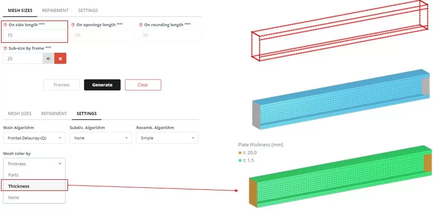
Step 2. Meshing
Navigate to the ‘Meshing’ menu. Set the FE element size to 15 mm, then click the ‘Generate’ button. The color of mesh can by updated by the plate thickness (‘SETTINGS’ > ‘Mesh color by’)
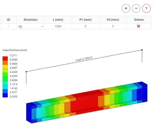
Step 3. Imperfections
Navigate to the ‘Imperfection’ menu. Set the settings, then click the Preview’ button.
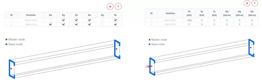
Step 4. Boundaries and Load
Navigate to the ‘Boundaries‘ > ‘Rigid Ends’ menu. Set the end boundary constrains. Navigate to the ‘Loads‘ > ‘Rigid Ends’ menu. Apply an axial load of 1000 kN to the left end of the member for compression.
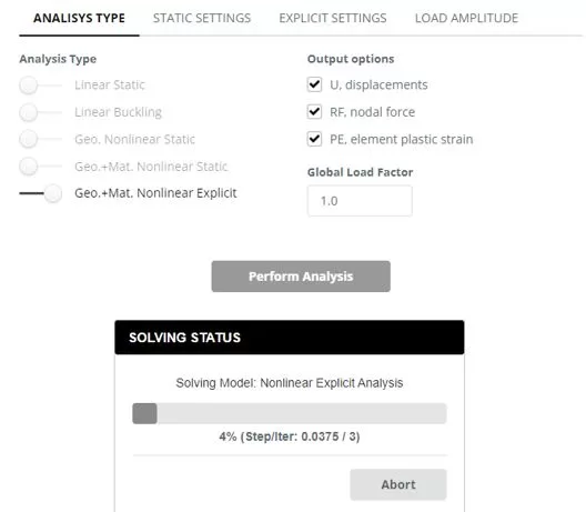
Step 5. Analysis and Load-Displacement tracking
Navigate to the ‘Analysis‘ menu. Select Nonlinear Explicit including geometry and material nonlinearity. Click ‘Perform Analysis’ button.
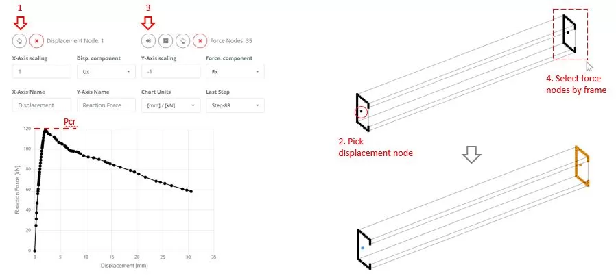
While the analysis is in progress, navigate to ‘Chart’ menu. First, select a node to measure the Ux displacement (steps 1 and 2). Then, using frame selection, choose nodes from which to extract the Rx reaction forces (steps 3 and 4). Monitor the chart’s changes to identify the critical force (Pcr) that leads the structure to failure. Terminate the ongoing analysis once the failure state is detected.
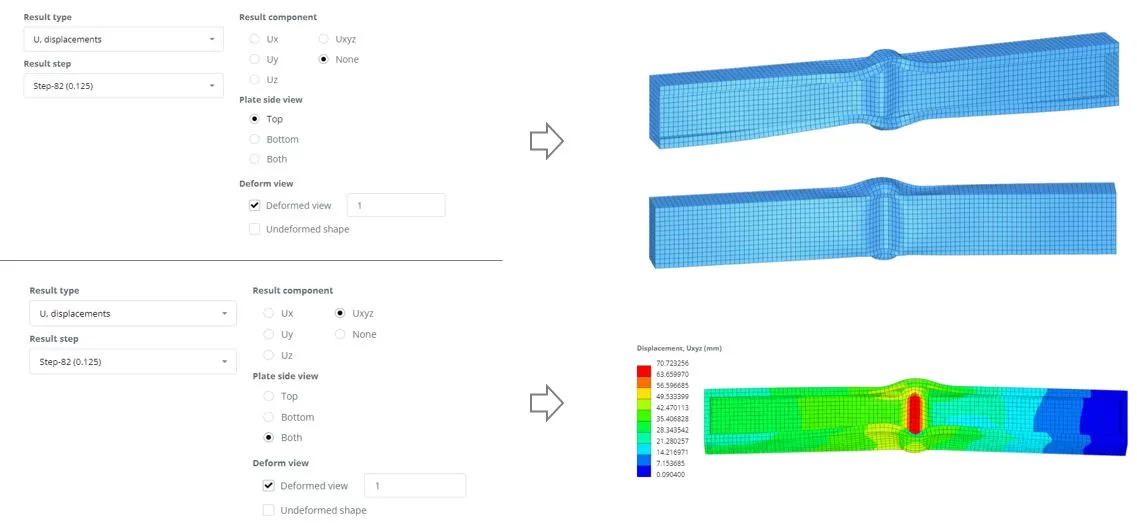
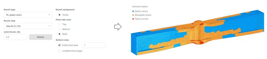
Step 6. Results
Navigate to the ‘Results’ menu, choose your preferred results options, and click ‘Display’ to view the deformed state of the model.
SkyCiv Structural Engineering Software
If you haven’t already, sign up for free with SkyCiv today and unlock powerful structural analysis and design tools to accelerate your engineering projects!