Definition of frequency analysis?
When designing buildings, there are two types of loads to consider: static and dynamic. For the first one, it is only needed to calculate the direct response of the structure against the permanent loads applied in terms of displacement and stresses. This can be achieved using the Stiffness or the Finite Element Method.
In the case of dynamic analysis, it is more challenging to consider the range of possible variations in the structure’s response due to time-dependent loads. Therefore, some new tools or functions become essential to include in the analysis. So, frequency analysis, a fundamental method in vibration mechanics, arises.
This method obtains the variation in time of the structure motion due to the dynamics loads applied. More specifically, this implies using the natural properties of vibration of the structural system to calculate internal forces, displacements, stability problems, etc.
For more information on the topic, we suggest reading a SkyCiv article that briefly explains how to perform a Dynamic Frequency Analysis using SkyCiv Structural Analysis Software.
Why is the frequency analysis relevant for design?
The best way to measure the importance of frequency analysis in a design is to watch the case of some structures that have failed due to bad dynamic behavior. One famous bridge in North America is the Tacoma Narrows, which finally collapsed after wind-induced sustained periodic vibrations. The following images will show the increased displacement along the bridge just before collapse, primarily focused on the roadway:
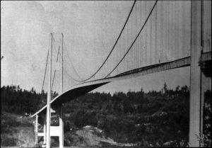
Figure i. Lateral torsional vibrations in Tacoma Narrows Bridge

Figure ii. Increased displacement on Bridge before the collapse.

Figure iii. Catastrophic Bridge Collapse
In this case study, a proper frequency analysis was not performed and the structure was not adequately designed to consider the structure’s natural frequency.
Simple pendulum
The frequency analysis studies the different forms a structure develops when it is subjected to external dynamic actions. This is why you get several different modes. Then using these forms, we can establish the structure’s element sizes through the internal forces required to guarantee the equilibrium.
Before going deeper into technical and mathematical considerations for frequency analysis, review the next simple system of a pendulum column shown in figure iv.
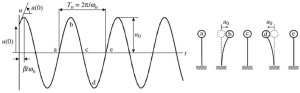
Figure iv. The dynamic response of a free vibration pendulum system
Using a simple analysis as indicated in the last image, we can define the motion of the top mass for the pendulum column every time. The main goal of this article will be to cover the frequency analysis for two typical cases, single and multiple degrees of freedom.
Single degree of freedom
This particular case is the simplest for dynamic analysis. The behavior is described using D’Alembert’s equilibrium law, an extension of the second Newton’s law.
The following figure shows the elements of the SDOF system, stiffness (k), damping (c), and mass source (m) for inertial forces. The time-varying external force applied onto the mass is represented by \({p(t)}\).
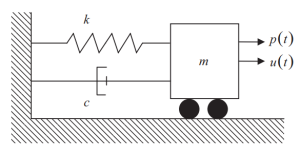
Figure 1. Single Degree of Freedom (SDOF) System. (Kausel, 2017, page 56)
All elements have to satisfy the dynamic equilibrium condition:
\({m}{\ddot{u}}+{c}{\dot{u}}+{k}{u}={p(t)}\)
This is a linear second-order differential equation, and its solution has two components:
\({u(t)}={u}_{h}(t)+{u}_{p}(t)\)
Where:
- \({u(t)}\) is the absolute displacement.
- \({u}_{h}(t)\) is the homogeneous solution, generally involving the free vibration case.
- \({u}_{p}(t)\) is the particular solution according to the excitation applied.
We will focus only on the homogeneous solution to describe vibration behavior and the most critical dynamic characteristics a structure has.
Let’s define the following terms:
\({\omega_{n}}={\sqrt(\frac {k}{m})}\) Angular frequency
\({\xi}={\frac{c}{{2}{m}{\omega_n}}}={\frac{c}{{2}{\sqrt(\frac {k}{m})}}}\) Fraction of critical damping
When the fraction of critical damping is less than 1, the vibration case will be underdamped; that is, there will be completed cycles before the motion stops.
The solution is of the following general form
\({u_h}={e^{{-\xi}{\omega_{n}}{t}}}{[{A}{cos}{\omega_d}{t}+{B}{sin}{\omega_d}{t}]}\)
Where:
- A and B are integration constants that depend on motion’s initial conditions.
- \({\omega_d}={\omega_n}{\sqrt({{1}-{\xi^2}})}\) is the damped angular frequency
Once evaluating A and B constants, the general solution for the undamped case is
\({u_h}={e^{{-\xi}{\omega_{n}}{t}}}{[{u_0}{cos}{\omega_d}{t}+{\frac{{\dot{u_0}}+{\xi}{\omega_n}{u_0}}{\omega_d}}{sin}{\omega_d}{t}]}\)
Where:
- \({u_0}\) is the mass initial displacement
- \(\dot{u_0}\) is the mass initial velocity
If we plot the solution with some values of initial conditions, we will obtain the following figure.
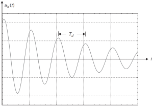
Figure 2. Displacement results in a homogeneous part of the solution in a subcritical damped case. (Kausel, 2017, page 58)
In the other case, it’s crucial to analyze what happens when the fraction of critical damping has a value of 1. \({\xi}=1\). This condition implies a structure with complete damping.
The equation to use is
\({u_h}={e^{{-\omega_{n}}{t}}}{\{u_0+({\dot{u_0}}+{\omega_n}{u_0}){t}}\}\)
And their graph showing different cases of initial conditions is in the following image.
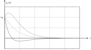
Figure 3. Displacement results in a homogeneous part of the solution in a critically damped case. (Kausel, 2017, page 58)
Response parameters
The previous section helped us to define the solution for free dynamic vibration in an SDOF system. The two main parameters are natural frequency \(\omega_n\) which indicates how the structure will vibrate on its own, and the fraction of critical damping \(\xi\), which defines the velocity in decaying vibrations.
Generally, structures have low damping with a maximum value of \(\xi\)=10 %. If we evaluate the damped natural frequency using this value, the result is \({\omega_d}=0.995{\omega_n}\). So, it is recommended to use \({\omega_d}{\thickapprox}{\omega_n}\).
We can summarize the dynamic properties in the following table.
| Angular frequency (rad/s) | Natural frequency (Hz) | Natural period (s) | |
|---|---|---|---|
| Angular frequency \({\omega_n}\) | \({\omega_n}\) | \(2{\pi}{f_n}\) | \(\frac{2{\pi}}{T_n}\) |
| Natural frequency \({f_n}\) | \(\frac{\omega_n}{2{\pi}}\) | \(f_n\) | \(\frac{1}{T_n}\) |
| Natural period \({T_n}\) | \(\frac{2{\pi}}{\omega_n}\) | \(\frac{1}{f_n}\) | \(T_n\) |
Table 1. Relationship between angular frequency, natural frequency, and period (Kausel, 2017, page 60)
Multiple degrees of freedom
When many masses exist in a structure, we have to define multiple coordinates to describe the position at any time for these masses. One particular and obvious example is shown in the following figure, consisting of a complex pendulum where different angles are needed to establish the position at every moment of motion.
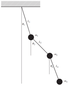
Figure 4. Pendulum with multiple masses. (Kausel, 2017, page 53)
In this section, we analyze structures’ general dynamic response using the extension of properties frequency analysis for multiple degrees of freedom.
It’s imperative to be aware of the modeling process when dealing with an actual structure. The following images describe the required steps to construct a mathematical model ready to apply the frequency analysis to describe its dynamic response.
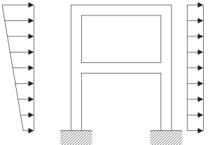
Figure 5. Physical model of a continuum structural frame. (Kausel, 2017, page 23)
The first step involves lumping masses at every level intersection of beams and columns. Each node has three possible movements, two linear displacements, and one rotation. To be consistent in the analysis, masses and polar inertial properties must be considered.
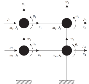
Figure 6. Lumped masses at nodes with displacement and rotation degrees of freedom. Discrete System. (Kausel, 2017, page 23)
The static condensation method can help reduce the complexity of analysis, neglecting rotational and translational inertia.
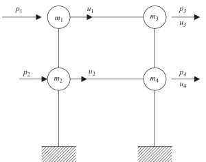
Figure 7. Static condensation of the degree of freedom to only horizontal displacement. (Kausel, 2017, page 23)
In the last step, we can lump in only two nodes the horizontal motion for this frame example.
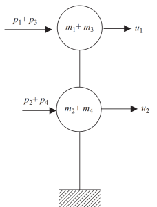
Figure 8. Final static condensation to two nodes and horizontal displacement degree of freedom. (Kausel, 2017, page 24)
As we did in the previous section with the SDOF system, we will develop the solution to the motion equation for multiple degrees of freedom.
The motion equation writes in matrix form as
\([M]\{\ddot{u}\} + [C]\{\dot{u}\}+[K]\{u\}={p(t)}\)
Where:
- \([M]\) is the mass matrix
- \([C]\) is Coulumb’s damping matrix
- \([K]\) is the stiffness matrix
We have to study the free vibration solution to obtain the response parameters. There is no damping and force applied to the system, only the initial conditions to be evaluated.
\([M]\{\ddot{u}\} +[K]\{u\}={0}\)
In analogy to the first case for an SDOF, we can test a sinusoidal solution of the form.
\({u(t)}={\phi}{({a}{cos}{\omega}{t}+{b}{sin}{\omega}{t})}\)
\({\ddot{u}{(t)}}={-{\omega}^2}{\phi}{({a}{cos}{\omega}{t}+{b}{sin}{\omega}{t})}\)
In which the vector \(\phi\) is a shape vector that does not time depending. The coefficients “a” and “b” are constants obtained when evaluating initial conditions.
After substituting both expressions for the test solution into the motion equation, we obtain the linear eigenvalue-eigenvector problem:
\([K]{\phi}={{\omega}^2}[M]{\phi}\)
Where:
- \({{\omega}^2}\) is the set of eigenvalues
- \({\phi}\) is the set of eigenvectors
The solution to this classic problem for the frame example in the latest figures shows how masses will vibrate. This means that every mass will move in a horizontal direction according to the value of eigenvectors.
Look at the following image of this behavior.
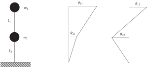
Figure No.9. Frequency analysis showing the two eigenvectors results. (Kausel, 2017, Page 135)
SkyCiv Structural 3D
Perform frequency analysis for your structures with SkyCiv Structural 3D. Sign up today to get started!
References:
- Eduardo Kausel, (2017). “Advanced Structural Dynamics” 1st edition, Cambridge University Press