In steel connection design, bolts are usually designed as a bolt group that will act as one body to resist a given load. The strength of a bolt group is usually calculated by the controlling strength of its most critical bolt. The direct loads are distributed among the total number of bolts, while the induced moment due to the loads’ eccentricity is distributed in relation to the bolt group’s moment of inertia and distance from the centroid. This analysis is called the elastic analysis. Due to its simplified and conservative assumptions on the load distribution, it often yields over-designed bolted connections.
When talking about value-engineering and economical designs, the inelastic approach is preferred by most manufacturers. It requires a lesser number of bolts for the same magnitude of loads. To do the inelastic approach, the instantaneous center of rotation (ICOR) method using iterations is the best way.
In this article, we will demonstrate how to calculate the strength of a bolted connection using the ICOR method. The reactions per bolt will be calculated using Equation (7-1) on pages 7-7 of the AISC 15th Edition Manual. This will then be used to check if the assumed location of the instantaneous center of the bolt group is correct. Finally, once we have the correct IC location, we will then calculate the bolt group coefficient C to determine its strength.
The use of the ICOR method in getting the bolt group coefficient is a long process as it requires a trial and error method of getting the Instantaneous Center (IC) location. Nowadays, with the use of computer solvers, the IC of a bolt group can be easily calculated using programmed iterations. SkyCiv Bolt Group Solver uses a fast iteration method to determine the IC location and the bolt group coefficient in just seconds. It is currently implemented in the AS 4100 design code but will be integrated into the rest of the design codes soon.
Getting the Bolt Group Properties
Let’s start our simple analysis on a bolt group of four bolts loaded with an eccentric vertical shear load of 10 kips. The eccentricity of the load along x axis is 4 inches to the right of the bolt group. The angle from the vertical is zero and the eccentricity along y-axis is zero.
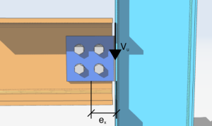
\(V_{u} = 10kips \)
\(\theta = 0 deg\)
\(e_{x} = 4 in\)
\(e_{y} = 0in\)
The first thing to do is to get the coordinates of all the bolts in our bolt group. The use of visual guides and tables is highly recommended.
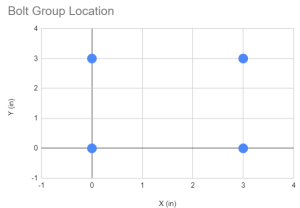
| Bolt ID | X (in) | Y (in) |
| 1 | 0 | 0 |
| 2 | 0 | 3 |
| 3 | 3 | 0 |
| 4 | 3 | 3 |
To get the centroid of the bolt group along the x- and y-axes, we need the formula below.
Let \(n \) = total number of bolts
\(X_{CG} = \frac{\sum X}{n}\)
\(Y_{CG} = \frac{\sum Y}{n} \)
Then, our solution is:
\(X_{CG} = \frac{\sum X}{n} = \frac{0 in + 0 in + 3 in + 3 in}{4} = 1.5 in\)
\(Y_{CG} = \frac{\sum Y}{n} = \frac{0 in + 3 in + 0 in + 3 in}{4} = 1.5 in\)
Assume the location of the I.C.
After getting the centroid, we will assume the location of the instantaneous center \(IC\). As a first try, we can assume that the IC is located at the geometric centroid of the bolt group.
So, assume
\(X_{IC} = X_{CG} = 1.5 in\)
\(Y_{IC} = Y_{CG} = 1.5 in\)
Then, we tabulate the displacement of each bolt to the location of the IC. We can simply do this by getting the distance along x and distance along y first, then get its displacement
| Bolt ID | cx (in) | cy (in) | c (in) |
| 1 | -1.5 | -1.5 | 2.121 |
| 2 | -1.5 | 1.5 | 2.121 |
| 3 | 1.5 | -1.5 | 2.121 |
| 4 | 1.5 | 1.5 | 2.121 |
Where,
\(c_{x} = X_{i} – X_{IC}\)
\(c_{y} = Y_{i} – Y_{IC}\)
\(c = \sqrt{{\left(c_{x} \right)}^{2} + {\left(c_{y} \right)}^{2}}\)
For Bolt No. 1, our solution is
\(c_{x} = 0in – 1.5 in = -1.5 in\)
\(c_{y} = 0in – 1.5 in = -1.5 in\)
\(c = \sqrt{{\left( -1.5 in \right)}^{2} + {\left( -1.5 in \right)}^{2}} = 2.121in\)
Calculate the deformation per bolt wrt distance from IC
Consequently, after getting the bolt distances from the assumed IC location, we then calculate the deformation of each bolt as a function of its distance.
The maximum deformation per bolt, set to \(\Delta_{max} = 0.34 in\), is based on experimental data for an ASTM bolt as described in AISC page 7-8. By using linear proportion, and setting \(\Delta_{max} = 0.34 in\), we can calculate the deformation of an individual bolt relative to its portion to the maximum distance \(c_{max}\). The equation for getting is shown below.
\(\Delta_{1} = 0.34in \times \left( \frac{c}{c_{max}}\right) \)
For Bolt No. 1, the deformation is
\(\Delta_{1} = 0.34in \times \left( \frac{2.121 in}{2.121 in}\right)\)
For the rest of the bolts, the calculated deformations are tabulated below.
| Bolt ID | \(\Delta\) (in) |
| 1 | 0.34 |
| 2 | 0.34 |
| 3 | 0.34 |
| 4 | 0.34 |
Get the reactions per bolt
Once we have the deformation per bolt, we can then use AISC 15th Ed. Eq (7-1) to get the reactions per bolt.
\(R = R_{ult} \left ( 1 – e^{-10\Delta}\right )^{0.55}\)
The \(R_{ult}\) in the equation is the assumed ultimate load on a bolt, which we can set as the bolt shear strength.
\(R_{ult} = \phi R_{n} \)
For our example, we will use a bolt shear strength of \(24.4 kip\). It is also permissible to use another value as this will just cancel out when we calculate the bolt group coefficient \(C\) later on.
For Bolt No. 1, the calculated reaction is
\(R = R_{ult} \left ( 1 – e^{-10\Delta}\right )^{0.55}\)
\(R = 24.4 kip \left ( 1 – e^{-10 \times \left ( 0.34 in \right )}\right )^{0.55}\)
\(R = 23.949 kip\)
For the rest of the bolts, the calculated reactions are as follows. At the same time, the components of bolt reaction \(R\) along x and y are also shown.
| Bolt ID | R (kip) | Rx (kip) | Ry (kip) |
| 1 | 23.949 | 16.937 | -16.937 |
| 2 | 23.949 | -16.937 | 16.937 |
| 3 | 23.949 | 16.937 | -16.937 |
| 4 | 23.949 | -16.937 | 16.937 |
| ⅀Rx = 0 | ⅀Ry = 0 |
For Bolt No.1, the solutions for getting the x and y components are shown below.
\(R_{x} = -R \left ( \frac{c_{y}}{c} \right ) = -23.949 \times \left ( \frac{-1.5in}{2.121in} \right ) = 23.949 kip\)
\(R_{y} = R \left ( \frac{c_{x}}{c} \right ) = 23.949 \times \left ( \frac{1.5in}{2.121in} \right ) = 23.949 kip\)
Moreover, we should get the induced moment load per bolt due to the eccentricity. To calculate this, we use the components \(R_{x}\) and \(R_{y}\) and multiply them with the eccentricities \(c_{y}\) and \(c_{x}\), respectively.
For Bolt No.1, the moment reaction to the IC is
\(M_{r} = -R_{x}c_{y} + -R_{y}c_{x} \)
\(M_{r} = -16.937 kip \times \left ( -1.5in \right) + -16.937 kip \times \left ( -1.5 in \right ) \)
\(M_{r} = 50.811 kip-in\)
For the rest of the bolts, the corresponding moment reactions are tabulated below.
| Bolt ID | Mr (kip-in) |
| 1 | 50.811 |
| 2 | 0 |
| 3 | 0 |
| 4 | 50.811 |
| ⅀Mr = 101.622 |
Verifying the IC location
Now that we have the shear and moment reactions per bolt, we will use that to determine the amount of Pu load that this bolt group resists. To do this, we will get the resultant of the sum of all reactions along x and sum of all reactions along y.
From the previous section, we have calculated that
\(\sum R_{x}=0kip\)
and
\(\sum R_{y}=0kip\)
So,
\(P_{u} = \sqrt{{\left( \sum R_{x} \right)}^{2} + {\left( \sum R_{y} \right)}^{2}} = 0 kip\)
Since the resulting load \(P_{u} = 0kip\), we can decide at this point to not proceed with the verification since our data will just be zero. We can also infer that the first assumed location of I.C., which is at the centroid of the bolt group, is incorrect. However, for the purpose of this discussion, we will proceed with the steps below.
\(P_{ux} = -P_{u}sin\left ( \theta \right ) = 0 kip \)
\(P_{uy} = -P_{u}cos\left ( \theta \right ) = 0 kip \)
\(M_{u} = -P_{ux}\left ( Y_{CG} + e_{y} – Y_{IC} \right ) + -P_{uy} \left (X_{CG} + e_{x} – X_{IC} \right ) = 0 kip \)
Since,
\(P_{ux} \neq \sum R_{x} \)
\(P_{uy} \neq \sum R_{y} \)
\(M_{u} \neq \sum M_{r} \)
Therefore, the assumed location of I.C. is incorrect. We can now proceed with the next assumed location.
SkyCiv has full integration of the bolt group calculation into the Australian Standard Module. Want to try our connection design software?
Second Iteration
For our second iteration, let us assume that the I.C. is located at the coordinates shown below.
Assume
\(X_{IC} = 0.062 in\)
\(Y_{IC} = 1.5 in\)
Then, let’s do the steps that we did in our first iteration. In summary, the table below will show the coordinates, the distance of each bolt from the assumed I.C, and the corresponding deformation with respect to the distance.
| Bolt ID | X (in) | Y (in) | cx (in) | cy (in) | c (in) | \(\Delta\) (in) |
| 1 | 0 | 0 | -0.062 | -1.5 | 1.501 | 0.155 |
| 2 | 0 | 3 | -0.062 | 1.5 | 1.501 | 0.155 |
| 3 | 3 | 0 | 2.938 | -1.5 | 3.299 | 0.34 |
| 4 | 3 | 3 | 2.938 | 1.5 | 3.299 | 0.34 |
Note that the calculated centroid of the bolt group is still the same since nothing has changed on the bolt coordinates.
\(X_{CG} = 1.5 in\)
\(Y_{CG} = 1.5 in\)
Then, we calculate the reactions along x, reactions along y, and the corresponding moment. The values are tabulated below.
| Bolt ID | R (kip) | Rx (kip) | Ry (kip) | Mr (kip-in) |
| 1 | 21.4 | 21.4 | -0.9 | 32.1 |
| 2 | 21.4 | -21.4 | -0.9 | 32.1 |
| 3 | 23.9 | 10.9 | 21.3 | 79.0 |
| 4 | 23.9 | -10.9 | 21.3 | 79.0 |
| ⅀Rx = 0 | ⅀Ry = 41 | ⅀Mr = 222 |
Next, we determine the resultant load of all the reactions along x and y.
\(P_{u} = \sqrt{{\left( \sum R_{x} \right)}^{2} + {\left( \sum R_{y} \right)}^{2}}\)
\(P_{u} = \sqrt{{\left( 0 kip\right)}^{2} + {\left( 40.703 kip\right)}^{2}}\)
\(P_{u} = 40.703 kip\)
Then, the components of the resultant load based on the given \(\theta\) is shown below.
\(P_{ux} = -P_{u}sin \left ( \theta \right ) = -41kip \times sin \left ( 0 deg \right )= 0 kip\)
\(P_{uy} = -P_{u}cos \left ( \theta \right ) = -41kip \times cos \left ( 0 deg \right )= -41 kip\)
We will then use these components to solve for the moment load about the assumed I.C.
\(M_{u} = -P_{ux} \left ( Y_{CG} + e_{y} – Y_{IC} \right) + P_{uy} \left ( X_{CG} + e_{x} – X_{IC} \right)\)
\(M_{u} = -0 kip \left ( 1.5 in +0 in – 1.5 in \right) + 41 kip \left ( 1.5 in +4 in – 0.06 in \right)\)
\(M_{u} = -222 kip-in\)
Next, let us compare the calculated Pux, Pux, and Mu to the reactions of the bolt group.
\(P_{ux} \approx – \sum R_{x}\)
\(P_{uy} \approx – \sum R_{y}\)
\(M_{u} \approx – \sum M_{u}\)
Since the left hand side is almost equal to the right hand side of the equation, we can say that the assumed location of I.C. is correct!
Solving for C coefficient
Once the I.C. location is determined, we can now get the bolt group coefficient C with the formula below.
\(C = \frac{P_{u}}{\phi R_{n}} = \frac{40.703 kip}{24.4 kip} = 1.668\)
Free Bolt Group Calculator
Check how we design our bolted connections with this approach using our Free Steel Connection Design Calculator! For more functionality, sign up for our Structural 3D software today to get started!