Estimating Pile Capacity
Estimating the Pile load-carrying capacity is necessary to determine the ultimate axial load that the pile can carry. The ultimate load capacity of the pile (Qu) is equivalent to the sum of end-bearing capacity (Qp) and frictional resistance (Qs), represented by Fig. 1 and Eq. 1. Numerous published studies and practices determine the pile’s end-bearing capacity and frictional resistance. This article focuses on various methods to estimate the ultimate pile capacity.
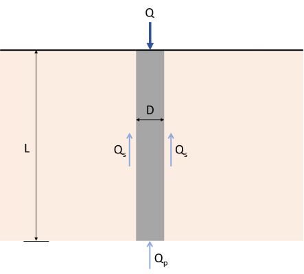
\( {Q}_{u} = {Q}_{p} + {Q}_{s} \) (1)
Qu : Ultimate load-carrying capacity
Qp : End-bearing load capacity
Qs : Skin-frictional resistance
Universal equations for Qp and Qs
\( {Q}_{p} = {A}_{p} \times {q}_{p} \) (2)
\( {q}_{p} = (c \times {N}_{c}) + (q’ \times {N}_{q}) + (\gamma \times D \times {N}_{\gamma}) \) (3)
\( {Q}_{p} = {A}_{p} \times[ (c \times {N}_{c}) + (q’ \times {N}_{q}) ] \) (4)
The total frictional resistance of the pile, which is developed along its length, can be calculated using this equation:
\( {Q}_{s} = ∑ (p × ΔL × f) \) (5)
p: Perimeter of the pile
ΔL: Incremental pile length over which p and f are taken
f: Unit frictional resistance at any depth
Methods for Estimating Qp
Meyerhof’s Method
Sandy Soil
According to Meyerhof, the unit point resistance (qp) of piles in sand generally increases with the embedment length until it reaches its maximum value when the embedment ratio (L/D) reaches a critical value. Critical embedment ratio (L/D)cr usually varies from 16 to 18. In this method, piles in the sand are assumed to have zero cohesion (c ≈ 0), and the unit point resistance should not exceed limiting point resistance (ql), which is given by Eq. 7. The bearing capacity factor (Nq) values are directly proportional to the soil friction angle of the bearing stratum (Table 1). Based on Meyerhof’s theory, the universal equation for Qp (Eq.4) can be simplified to:
\( {Q}_{p} = {A}_{p} \times (q’ \times {N}_{q}) \leq ({A}_{p} \times {q}_{l}) \) (6)
\( {q}_{l} = 0.5 \times {p}_{a} \times {N}_{q} \times tan (\phi’) \) (7)
ql : Limiting point resistance
pa: Atmospheric pressure (≈100 kN/m2)
\( \phi’\): Effective soil friction angle at the tip of the pile
Table 1: Interpolated values of Nq (Meyerhof’s theory)
Clay Soil
Equation 4 can also calculate the end-bearing capacity of piles in clay or cohesive soils (φ ≈ 0). Since soil friction angle is neglected and the bearing capacity factor (Nc) has a constant value of 9 for cohesive soils, Eq.4 can be written as:
\( {Q}_{p} = {A}_{p} \times c \times {N}_{c} = 9 \times c \times {A}_{p} \) (8)
Vesic’s Method
Vesic’s method of calculating end-bearing capacity on sandy or clayey soils is based on his theory of the expansion of cavities.
Sandy Soil
Based on his theory, end-bearing capacity of piles in sand can be estimated using the following equations:
\( {Q}_{p} = {A}_{p} \times \bar{\sigma’}_{o} \times {N}_{\sigma} \) (9)
\(\bar{\sigma’}_{o} = \frac{1 + (2 \times {K}_{o})}{3} \times q’\) (10)
\( {K}_{o} = 1 – sin \phi’\) (11)
\( {N}_{\sigma} = \frac{3 \times {N}_{q}}{1 + (2 \times {K}_{o})} \) (12)
\(\bar{\sigma’}_{o} \) : Mean effective normal ground stress at the level of the pile point
Ko: Earth pressure coefficient at rest
Nσ: Bearing capacity factor
Clay Soil
Same with Meyerhof’s method, Eq. 4 is also applicable to calculate the end-bearing capacity of piles in clay. However, the value of the bearing capacity factor (Nc) is a factor of rigidty index (Ir). According to his theory of expansion of cavities, Nc and Ir can be estimated by:
\( {N}_{c} = (\frac{4}{3}) \times [ln({I}_{r}) + 1] + \frac{\pi}{2} + 1 \) (13)
\( {I}_{r} = \frac{{E}_{s}}{3 \times c} \) (For φ ≈ 0)(14)
Ir: Rigidity index
Es: Modulus of elasticity of soil
Coyle and Castello’s Method (Sandy Soil)
Based on 24 large-scale field load tests of driven piles in sand, Coyle and Castello suggested that the end-bearing capacity of piles can be calculated using Eq.15. The values of the bearing capacity factor (Nq) is a factor of both embedment ratio (L/D) and the soil friction angle (φ’), as shown in Fig. 2
\( {Q}_{p} = {A}_{p} \times (q’ \times {N}_{q}) \) (15)
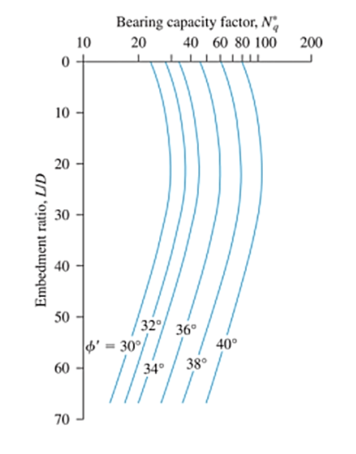
Figure 2: Variation of Nq with L/D & φ’ (Redrawn after Coyle & Castello, 1981)
Source: Das, Braja. Principles of Foundation Engineering (7th Edition, p.564)
Methods for Estimating Qs
Frictional Resistance of Piles in Sand
The unit frictional resistance of piles in sand, as shown in Eq. 5, considers multiple factors which are quite difficult to calculate. It includes the earth pressure coefficient (K) & soil-pile friction angle, which both have varying values depending on which approach to use or to the available soil data.
\( f = K\times {\sigma}_{o}’ \times tan (\delta) \) (15)
K: Effective earth pressure coefficient
σ’o: Effective vertical stress at the depth under consideration
δ: Soil-pile friction angle
The following are the different ways to estimate the effective earth pressure coefficient and soil-friction angle values. These variables are a factor of soil frictional angle (φ’) or pile type.
Effective earth pressure coefficient
The soil exerts lateral earth pressure to the pile surface. It is necessary to account for this pressure on the design or analysis for stability. The following are the different ways to determine the earth pressure coefficients to calculate the unit frictional resistance of piles in sand.
NAVFAC DM 7.2
| Pile Type | Compression | Uplift |
|---|---|---|
Table 2: Earth pressure coefficient, K (NAVFAC DM 7.2)
Average K Method
The earth pressure coefficient (K) can also be evaluated by taking the average of earth pressure coefficient at rest (K0), active earth pressure (Ka), and passive earth pressure (Kp), as shown from Equations 16-19.
\( K =\frac{{K}_{0} + {K}_{a} + {K}_{p}}{3} \) (16)
\( (K)_{0} =1 – sin \phi \) (17)
\( (K_{a} =1 – {tan}^{2}( \frac{45 – \phi}{2}) \) (18)
\( (K_{p} =1 + {tan}^{2}( \frac{45 + \phi}{2}) \) (19)
Mansur and Hunter (1970)
Based on different field load test results, Mansur and Hunter concluded the values of earth pressure coefficient with the corresponding pile types.
| Pile Type | K |
|---|---|
Table 3: Earth pressure coefficient, K (Mansur and Hunter, 1970)
Soil-pile Friction Angle
The friction angle between the soil and the surface of the pile is an essential aspect of foundation design. Practically, many engineers approximate this value as equal to 2/3 of the internal friction angle of the soil. However, based on the study of Coyle and Castello in 1981, the soil-pile friction angle is approximately equivalent to 80% of the internal friction angle of the soil. On the other hand, NAVFAC DM7.2 uses these values to estimate the friction angle between the soil and pile:
| Pile Type | δ |
|---|---|
Table 4: Soil-pile friction angle (δ) (NAVFAC DM 7.2)
Frictional Resistance of piles in Clay
Calculating the frictional resistance of piles in clayey soils can be as challenging as the one in sandy soils due to the introduction of new variables, which are also not as easy to determine. However, there are several available methods to obtain the values of these variables.
λ Method
Based on the study of Vijayvergiya and Focht in 1972, the total frictional resistance of piles in clay can be estimated by determining the average unit frictional resistance of the pile, as shown by Equations 20 and 21. λ values changes as the depth of the penetration of pile increases. Table 5 shows the variation of λ with the embedment length of the pile.
\( {f}_{av} = \lambda \times [\bar{\sigma’}_{o} +( 2 \times {c}_{u})] \) (20)
\({Q}_{s} = p \times L \times {f}_{av} \) (21)
\( \bar{\sigma’}_{o} \): Mean effective vertical stress for the entire embedment length
cu: Mean undrained shear strength
| L (m) | λ |
|---|---|
Table 5: Variation of λ with pile embedment length (L)
α Method
The α method suggests that unit frictional resistance of piles is equivalent to the product of the undrained cohesion of the soil layer and its corresponding empirical adhesion factor (α). Table 6 shows the corresponding value of the adhesion factor with the ratio of undrained cohesion and atmospheric pressure (cu/pa).
\(f = \alpha \times {c}_{u}\) (22)
Therefore, the total frictional resistance of pile in clay using this method can be re-written as:
\({Q}_{s} = \sum (f \times p \times \Delta L) = \sum (\alpha \times {c}_{u} \times p \times \Delta L)\) (23)
| cu/pa | α |
|---|---|
| 0.8 | |
pa = atmospheric pressure ≈ 100 kN/m2
Table 6: Variation of α (Terzaghi, Peck, and Mesri, 1996)
β Method
Pore water pressure around the pile increases when the pile is driven into saturated clays. This method, based on effective stress analysis, is suited for long-term (drained) analyses of the pile load capacity as it considers the gradual dissipation of the excess pore water pressure over time. According to Tomlinson (1971), piles driven in soft clays assume that failures occur in the remolded soil close to the pile surface. Based on Eq. 15, the term (K × tanδ) for unit frictional resistance of piles in sand shall be represented by β. The soil-friction angle (δ) shall be replaced by a remolded drained friction angle of the soil (Φ’R). Thus the unit frictional resistance of piles in clay is estimated to be equal to:
\(f = \beta \times {\sigma’}_{o}\) (24)
\(\beta = K \times tan {\Phi ‘}_{R}\) (25)
Conservatively, the earth pressure coefficient (K) is equivalent to the earth pressure coefficient at rest (K0) which varies for normally consolidated clays and overconsolidated clays, as shown in the following equations:
\( K = {K}_{0} = 1 – sin {\Phi ‘}_{R}\) (Normally consolidated clays) (26)
\( K = {K}_{0} = (1 – sin {\Phi ‘}_{R}) \times \sqrt(OCR)\) (Overconsolidated clays) (27)
OCR: Overconsolidation ratio
Want to try SkyCiv’s Foundation Design software? Our free tool allows users to perform load-carrying calculations without any download or installation!
References:
- Das, B.M. (2007). Principles of Foundation Engineering (7th Edition). Global Engineering
- Rajapakse, R. (2016). Pile Design and Construction Rule of Thumb (2nd Edition). Elsevier Inc.
- Tomlinson, M.J. (2004). Pile Design and Construction Practice (4th Edition). E & FN Spon.