Base Plate Design Example using EN 1993-1-8-2005, EN 1993-1-1-2005 and EN 1992-1-1-2004
Problem Statement
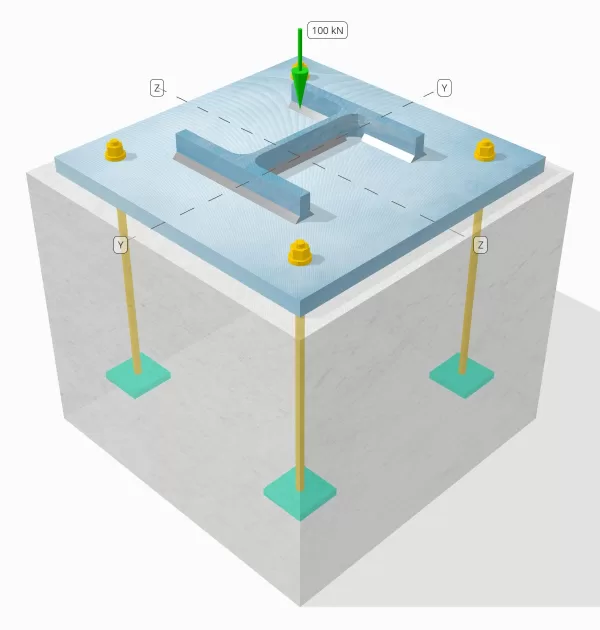
Determine whether the designed column-to-base plate connection is sufficient for a 100-kN compression load.
Given Data
Column:
Column section: HE 200 B
Column area: 7808 mm2
Column material: S235
Base Plate:
Base plate dimensions: 400 mm x 400 mm
Base plate thickness: 20 mm
Base plate material: S235
Grout:
Grout thickness: 20 mm
Concrete:
Concrete dimensions: 450 mm x 450 mm
Concrete thickness: 380 mm
Concrete material: C20/25
Welds:
Compression load transferred through welds only? NO
Model in SkyCiv Free Tool
Model the base plate design above using our free online tool today! No sign-up required.
Step-by-Step Calculations
Check #1: Calculate weld capacity
Since the compression load is not transferred through welds alone, a proper contact bearing surface is required to ensure that the load is transferred via bearing. Refer to EN 1090-2:2018 Clause 6.8 for contact bearing preparation.
Additionally, use minimum weld size specified in Eurocode.
Check #2: Calculate concrete bearing capacity and base plate yield capacity
The first step is to determine the design compressive strength of the joint, which depends on the geometry of the support (concrete) and the geometry of the loaded area (base plate).
We begin by calculating the alpha factor, which accounts for the diffusion of the concentrated force within the foundation.
According to EN 1992-1-1:2004, Clause 6.7, the alpha coefficient is the ratio of the loaded area to the maximum distribution area, which has a similar shape to the loaded area.
We will use the equation from Part 6.1 of Multi-Storey Steel Buildings Part 5 by Arcelor Mittal, Peiner Träger, and Corus to calculate the alpha factor.
\(
\alpha = \min \left(
1 + \frac{t_{\text{conc}}}{\max(L_{\text{bp}}, B_{\text{bp}})},
1 + 2 \left( \frac{e_h}{L_{\text{bp}}} \right),
1 + 2 \left( \frac{e_b}{B_{\text{bp}}} \right),
3
\right)
\)
\(
\alpha = \min \left(
1 + \frac{380 \, \text{mm}}{\max(400 \, \text{mm}, 400 \, \text{mm})},
1 + 2 \left( \frac{25 \, \text{mm}}{400 \, \text{mm}} \right),
1 + 2 \left( \frac{25 \, \text{mm}}{400 \, \text{mm}} \right),
3
\right)
\)
\(
\alpha = 1.125
\)
where,
\(
e_h = \frac{L_{\text{conc}} – L_{\text{bp}}}{2} = \frac{450 \, \text{mm} – 400 \, \text{mm}}{2} = 25 \, \text{mm}
\)
\(
e_b = \frac{B_{\text{conc}} – B_{\text{bp}}}{2} = \frac{450 \, \text{mm} – 400 \, \text{mm}}{2} = 25 \, \text{mm}
\)
Once the geometry is defined, we will then determine the compressive strength of the concrete using EN 1992-1-1:2004, Eq. 3.15.
\(
f_{cd} = \frac{\alpha_{cc} f_{ck}}{\gamma_C} = \frac{1 \times 20 \, \text{MPa}}{1.5} = 13.333 \, \text{MPa}
\)
Next, we assume a value for the beta coefficient. Since grout is present, beta value can be 2/3. We will calculate the design bearing strength of the joint using the combined formulas from EN 1993-1-8:2005 Eq. 6.6, and EN 1992-1-1:2004 Eq. 6.63.
\(
f_{jd} = \beta \alpha f_{cd} = 0.66667 \times 1.125 \times 13.333 \, \text{MPa} = 10 \, \text{MPa}
\)
The second part involves calculating the base plate yield capacity.
Since we already have the design bearing strength of the connection, we will use this to determine the smallest cantilever distance of the base plate that experiences the full bearing load. We will refer to the SCI P358 example on page 243 and EN 1993-1-1:2005 Clause 6.2.5.
\(
c = t_{\text{bp}} \sqrt{\frac{f_{y_{\text{bp}}}}{3 f_{jd} \gamma_{M0}}} = 20 \, \text{mm} \times \sqrt{\frac{225 \, \text{MPa}}{3 \times 10 \, \text{MPa} \times 1}} = 54.772 \, \text{mm}
\)
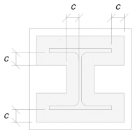
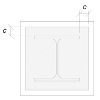
We will use this dimension to calculate the effective area of the base plate. The ‘c’ dimension we calculated may overlap or not overlap near the flange. If it overlaps, we will assume the section to be a rectangular section. If it does not overlap, we will take the shape of the column.
Without overlap
With overlap
We determined that the ‘c’ dimension does not overlap. Therefore, using SCI P358 pg. 243, the effective area is:
\(
A_e = 4c^2 + P_{\text{col}}c + A_{\text{col}} = 4 \times 54.772^2 \, \text{mm}^2 + 1182 \, \text{mm} \times 54.772 \, \text{mm} + 7808 \, \text{mm}^2 = 84549 \, \text{mm}^2
\)
It is important to note that the effective area should not be less than the base plate area.
Finally, we will use EN 1993-1-8:2005 Eq. 6.6, and EN 1992-1-1:2004, Eq. 6.63 to calculate the design bearing resistance of the base plate connection.
\(
N_{Rd} = \left( \min(A_e, A_0) \right) f_{jd} = \left( \min(84549 \, \text{mm}^2, 160000 \, \text{mm}^2) \right) \times 10 \, \text{MPa} = 845.49 \, \text{kN}
\)
Since 845.49 kN > 100 kN, the design is sufficient!
Design Summary
The SkyCiv Base Plate Design software can automatically generate a step-by-step calculation report for this design example. It also provides a summary of the checks performed and their resulting ratios, making the information easy to understand at a glance. Below is a sample summary table, which is included in the report.
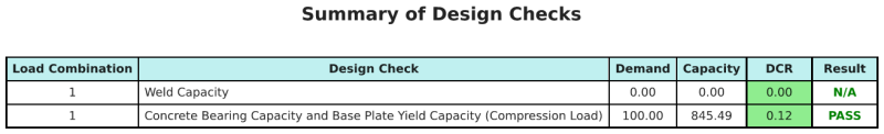
SkyCiv Sample Report
See the level of detail and clarity you can expect from a SkyCiv Base Plate Design Report. The report includes all key design checks, equations, and results presented in a clear and easy-to-read format. It is fully compliant with design standards. Click below to view a sample report generated using the SkyCiv Base Plate Calculator.
Purchase Base Plate Software
Purchase the full version of the base plate design module on its own without any other SkyCiv modules. This gives you a full set of results for Base Plate Design, including detailed reports and more functionality.