杭容量の見積り
杭が耐えられる最大軸方向荷重を決定するには、杭の耐荷重能力を見積もる必要があります。. 杭の極限耐荷重 (Qu) 端部支持力の合計に相当します (Qp) そして摩擦抵抗 (Q), 図で表される. 1 と等価. 1. 多数の発表された研究と実践により、杭の端部支持力と摩擦抵抗が決定されます。. この記事では、最終的な杭容量を見積もるためのさまざまな方法に焦点を当てます。.
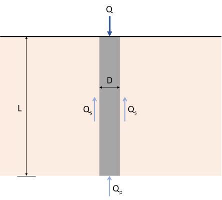
\( {Q}_{あなた} = {Q}_{p} + {Q}_{s} \) (1)
Qあなた : 究極の耐荷重能力
Qp : エンドベアリング耐荷重
Qs : 皮膚摩擦抵抗
Q の普遍方程式p とQs
\( {Q}_{p} = {あ}_{p} \回 {q}_{p} \) (2)
\( {q}_{p} = (c 回 {N}_{c}) + (q’ \回 {N}_{q}) + (\ガンマ times D times {N}_{\ガンマ}) \) (3)
\( {Q}_{p} = {あ}_{p} \回[ (c 回 {N}_{c}) + (q’ \回 {N}_{q}) ] \) (4)
パイルの総摩擦抵抗, その長さに沿って発達する, この式を使用して計算できます:
\( {Q}_{s} = ∑ (p×ΔL×f) \) (5)
p: 杭の周囲
L: p と f が取得される増分杭の長さ
f: あらゆる深さでのユニットの摩擦抵抗
Qp の推定方法
マイヤーホフ法
砂質土
マイヤーホフ氏によると, 単位点抵抗 (qp) 砂の中の杭の量は、一般に埋め込み長さとともに増加し、埋め込み率が最大値に達するまで増加します。 (L/D) 臨界値に達する. クリティカル埋め込み率 (L/D)cr 通常は~から変わります 16 に 18. この方法では, 砂の中の杭は凝集力がゼロであると仮定されます (c ≈ 0), 単位点抵抗は限界点抵抗を超えてはなりません (ql), これは式で与えられます. 7. 支持力係数 (Nq) 値は支持層の土壌摩擦角に正比例します。 (テーブル 1). マイヤーホフの理論に基づく, Q の普遍方程式p (式4) に簡略化できます:
\( {Q}_{p} = {あ}_{p} \回 (q’ \回 {N}_{q}) \leq ({あ}_{p} \回 {q}_{l}) \) (6)
\( {q}_{l} = 0.5 \回 {p}_{a} \回 {N}_{q} \日焼けの回数 (\ファイ) \) (7)
ql : 限界点抵抗
pa: 大気圧 (〜100kN/m2)
\( \ファイ): 杭先端の有効土壌摩擦角
テーブル 1: N の補間値q (マイヤーホフの理論)
粘土質の土壌
方程式 4 粘土または粘性土における杭の端部支持力も計算できます (φ ≈ 0). 土壌摩擦角は無視され支持力係数は無視されるため、 (Nc) の定数値があります 9 粘性土壌用, Eq.4 は次のように書くことができます。:
\( {Q}_{p} = {あ}_{p} \回 c 回 {N}_{c} = 9 \回 c 回 {あ}_{p} \) (8)
ヴェシッチのメソッド
砂質または粘土質の土壌における端部支持力を計算する Vesic の方法は、空洞の拡大に関する彼の理論に基づいています。.
砂質土
彼の理論に基づいて, 砂中の杭の端部支持力は、次の式を使用して推定できます。:
\( {Q}_{p} = {あ}_{p} \bar 倍{\シグマ'}_{の} \回 {N}_{\シグマ} \) (9)
\(\バー{\シグマ'}_{の} = frac{1 + (2 \回 {K}_{の})}{3} \q' 倍) (10)
\( {K}_{の} = 1 – sin \phi’\) (11)
\( {N}_{\シグマ} = frac{3 \回 {N}_{q}}{1 + (2 \回 {K}_{の})} \) (12)
\(\バー{\シグマ'}_{の} \) : 杭点レベルにおける平均有効垂直地盤応力
は: 静止時の土圧係数
Ns: 軸受容量係数
粘土質の土壌
マイヤーホフ法も同様, Eq. 4 粘土杭の端部耐力の計算にも適用可能. しかしながら, 支持力係数の値 (Nc) 剛性指数の要素です (私r). 彼の空洞拡大理論によると, Nc そして私r によって推定できます:
\( {N}_{c} = (\フラク{4}{3}) \回 [ln({私}_{r}) + 1] + \フラク{\パイ}{2} + 1 \) (13)
\( {私}_{r} = frac{{E}_{s}}{3 \c回} \) (φ ≈ の場合 0)(14)
私r: 剛性指数
Es: 土壌の弾性係数
コイルとカステッロの方法 (砂質土)
に基づく 24 砂中での打ち込み杭の大規模現場荷重試験, Coyle と Castello は、杭の端部耐力が Eq.15 を使用して計算できることを提案しました。. 支持力係数の値 (Nq) 両方の埋め込み率の係数です (L/D) と土壌摩擦角 (ピィ), 図に示すように. 2
\( {Q}_{p} = {あ}_{p} \回 (q’ \回 {N}_{q}) \) (15)
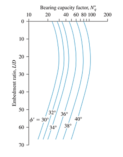
図 2: L/DによるNqの変化 & ファイ’ (コイルの後に再描画 & カステッロ, 1981)
ソース: それか, ブラジャ. 基礎工学の原則 (7第版, p.564)
Qの推定方法
砂中の杭の摩擦抵抗
砂中の杭の単位摩擦抵抗, 式に示すように. 5, 計算が非常に難しい複数の要素を考慮します. 土圧係数を含みます (K) & 土と杭の摩擦角, どちらも、使用するアプローチまたは利用可能な土壌データに応じて値が異なります。.
\( f = K回 {\シグマ}_{の}’ \日焼けの回数 (\デルタ) \) (15)
K: 有効土圧係数
σ’の: 考慮中の深さでの有効垂直応力
NS: 土と杭の摩擦角
以下は、有効土圧係数と土壌摩擦角の値を推定するさまざまな方法です。. これらの変数は、土壌摩擦角の要因です (ピィ) またはパイルタイプ.
有効土圧係数
土壌は杭表面に横方向の土圧を及ぼします. 安定性を確保するには、設計または解析に対するこのプレッシャーを考慮する必要があります。. 以下は、砂中の杭の単位摩擦抵抗を計算するための土圧係数を決定するさまざまな方法です。.
NAVFAC DM 7.2
| 杭タイプ | 圧縮 | 隆起 |
|---|---|---|
テーブル 2: 土圧係数, K (NAVFAC DM 7.2)
平均K法
土圧係数 (K) 静止時の土圧係数の平均をとることでも評価可能 (K0), 活動土圧 (Ka), および受動的土圧 (Kp), 方程式からわかるように 16-19.
\( K =frac{{K}_{0} + {K}_{a} + {K}_{p}}{3} \) (16)
\( (K)_{0} =1 – 罪 phi \) (17)
\( (K_{a} =1 – {黄褐色}^{2}( \フラク{45 – \ファイ}{2}) \) (18)
\( (K_{p} =1 + {黄褐色}^{2}( \フラク{45 + \ファイ}{2}) \) (19)
マンスールとハンター (1970)
さまざまなフィールド負荷テストの結果に基づく, Mansur と Hunter は、対応する杭の種類に応じた土圧係数の値を結論付けました。.
| 杭タイプ | K |
|---|---|
テーブル 3: 土圧係数, K (マンスールとハンター, 1970)
土と山の摩擦角
土壌と杭の表面の間の摩擦角は基礎設計の重要な要素です. 特に, 多くのエンジニアは、この値を次のように近似します。 2/3 土壌の内部摩擦角の. しかしながら, コイルとカステッロの研究に基づいています。 1981, 土と山の摩擦角はほぼ次の値に相当します。 80% 土壌の内部摩擦角の. 一方, NAVFAC DM7.2 はこれらの値を使用して土壌と杭の間の摩擦角を推定します。:
| 杭タイプ | NS |
|---|---|
テーブル 4: 土と杭の摩擦角 (NS) (NAVFAC DM 7.2)
粘土杭の摩擦抵抗
粘土質土壌における杭の摩擦抵抗の計算は、新しい変数の導入により、砂質土壌におけるものと同様に困難になる可能性があります。, これも簡単に判断できません. しかしながら, これらの変数の値を取得するには、いくつかの方法があります。.
λ法
のヴィジャイヴェルギヤとフォクトの研究に基づいています。 1972, 粘土中の杭の合計摩擦抵抗は、杭の平均単位摩擦抵抗を決定することによって推定できます。, 式で示されるように 20 そして 21. 杭の貫入深さが深くなると、λの値が変化します. テーブル 5 杭の埋込み長さによるλの変化を示します。.
\( {f}_{の} = lambda times [\バー{\シグマ'}_{の} +( 2 \回 {c}_{あなた})] \) (20)
\({Q}_{s} = p times L times {f}_{の} \) (21)
\( \バー{\シグマ'}_{の} \): 埋め込み長さ全体の平均有効垂直応力
cあなた: 平均非排水せん断強度
| L (メートル) | λ |
|---|---|
テーブル 5: 杭埋入長さによるλの変化 (L)
α法
α法は、杭の単位摩擦抵抗が土壌層の非排水凝集力とそれに対応する経験的付着係数の積に等しいことを示唆しています。 (a). テーブル 6 非排水凝集力と大気圧の比に対応する粘着係数の値を示します (cあなた/pa).
\(f = alpha times {c}_{あなた}\) (22)
したがって, この方法を使用した粘土中の杭の合計摩擦抵抗は、次のように書き直すことができます。:
\({Q}_{s} = sum (f times p times Delta L) = sum (\アルファ 回 {c}_{あなた} \倍 p time Delta L)\) (23)
| cあなた/pa | a |
|---|---|
| 0.8 | |
pa =大気圧≈ 100 kN / m2
テーブル 6: αの変化 (テルツァーギ, ペック, とメスリ, 1996)
β法
杭が飽和粘土に打ち込まれると、杭周囲の間隙水圧が増加します. この方法, 有効応力解析に基づく, 長期に適しています (消耗した) 時間の経過とともに過剰間隙水圧が徐々に消散することを考慮した杭耐荷重の解析. トムリンソン氏によると (1971), 柔らかい粘土に打ち込まれた杭は、杭の表面近くの再成形された土壌で破損が発生すると想定されています。. 方程式に基づく. 15, 用語 (K×tanδ) 砂中の杭の単位摩擦抵抗はβで表されるものとする. 土壌摩擦角 (NS) 再成型された排水された土壌の摩擦角に置き換えられます。 (ファイ’R). したがって、粘土中の杭の単位摩擦抵抗は次のように推定されます。:
\(f = beta times {\シグマ'}_{の}\) (24)
\(\ベータ = K times タン {\ファイ '}_{R}\) (25)
保守的に, 土圧係数 (K) 静止時の土圧係数に相当します (K0) これは、正常に固化した粘土と過剰に固化した粘土で異なります。, 次の式に示すように:
\( K = {K}_{0} = 1 – それなし {\ファイ '}_{R}\) (通常は固まった粘土) (26)
\( K = {K}_{0} = (1 – それなし {\ファイ '}_{R}) \回 sqrt(OCR)\) (過圧密粘土) (27)
OCR: 過密比率
SkyCivのFoundationDesignソフトウェアを試してみたい? 私たちの無料ツールを使用すると、ユーザーはダウンロードやインストールなしで耐荷重計算を実行できます!
参考文献:
- それか, B.M. (2007). 基礎工学の原則 (7第版). グローバルエンジニアリング
- ラジャパクセ, R. (2016). 親指の杭の設計と建設のルール (2第2版). エルゼビア株式会社.
- トムリンソン, M.J. (2004). パイルの設計と建設の実践 (4第版). E & FNスポンサー.