Ορισμός ανάλυσης συχνότητας?
Κατά το σχεδιασμό κτιρίων, υπάρχουν δύο τύπους φορτίων να εξετάσει: στατική και δυναμική. Για το πρώτο, Χρειάζεται μόνο για τον υπολογισμό της άμεσης απόκρισης της κατασκευής στα μόνιμα φορτία που εφαρμόζονται ως προς τη μετατόπιση και τις τάσεις. Αυτό μπορεί να επιτευχθεί χρησιμοποιώντας τη μέθοδο της ακαμψίας ή της μεθόδου πεπερασμένων στοιχείων.
Στην περίπτωση της δυναμικής ανάλυσης, είναι πιο δύσκολο να εξεταστεί το εύρος των πιθανών διακυμάνσεων στην απόκριση της κατασκευής λόγω φορτίων που εξαρτώνται από το χρόνο. Επομένως, ορισμένα νέα εργαλεία ή λειτουργίες καθίστανται απαραίτητα για να συμπεριληφθούν στην ανάλυση. Έτσι, ανάλυση συχνότητας, μια θεμελιώδης μέθοδος στη μηχανική των κραδασμών, προκύπτει.
Αυτή η μέθοδος λαμβάνει τη διακύμανση του χρόνου της κίνησης της δομής λόγω των δυναμικών φορτίων που εφαρμόζονται. Πιο συγκεκριμένα, Αυτό συνεπάγεται τη χρήση των φυσικών ιδιοτήτων της δόνησης του δομικού συστήματος για τον υπολογισμό των εσωτερικών δυνάμεων, μετατοπίσεις, προβλήματα σταθερότητας, και τα λοιπά.
Για περισσότερες πληροφορίες σχετικά με το θέμα, προτείνουμε να διαβάσετε ένα άρθρο του SkyCiv που εξηγεί εν συντομία πώς να εκτελέσετε ένα Ανάλυση δυναμικής συχνότητας χρησιμοποιώντας Λογισμικό δομικής ανάλυσης SkyCiv.
Γιατί η ανάλυση συχνότητας είναι σχετική για το σχεδιασμό?
Ο καλύτερος τρόπος για να μετρήσετε τη σημασία της ανάλυσης συχνότητας σε ένα σχέδιο είναι να παρακολουθήσετε την περίπτωση ορισμένων δομών που απέτυχαν λόγω κακής δυναμικής συμπεριφοράς. Μια διάσημη γέφυρα στη Βόρεια Αμερική είναι η Tacoma Narrows, το οποίο τελικά κατέρρευσε μετά από συνεχείς περιοδικές δονήσεις που προκαλούνται από τον άνεμο. Οι παρακάτω εικόνες θα δείχνουν την αυξημένη μετατόπιση κατά μήκος της γέφυρας λίγο πριν την κατάρρευση, επικεντρώνεται κυρίως στο οδόστρωμα:
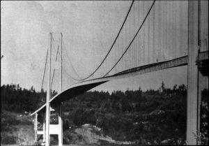
Εικόνα i. Πλευρικές στρεπτικές δονήσεις στη γέφυρα Tacoma Narrows Bridge

Εικόνα ii. Αυξημένη μετατόπιση στη Γέφυρα πριν από την κατάρρευση.
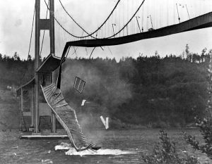
Εικόνα iii. Καταστροφική κατάρρευση γέφυρας
Σε αυτή τη μελέτη περίπτωσης, δεν πραγματοποιήθηκε σωστή ανάλυση συχνότητας και η δομή δεν σχεδιάστηκε επαρκώς ώστε να λαμβάνει υπόψη τη φυσική συχνότητα της δομής.
Απλό εκκρεμές
Η ανάλυση συχνότητας μελετά τις διαφορετικές μορφές που αναπτύσσει μια δομή όταν υπόκειται σε εξωτερικές δυναμικές ενέργειες. Αυτός είναι ο λόγος που παίρνετε πολλά διαφορετικά τρόπους λειτουργίας. Στη συνέχεια, χρησιμοποιώντας αυτές τις φόρμες, μπορούμε να καθορίσουμε τα μεγέθη των στοιχείων της δομής μέσω των εσωτερικών δυνάμεων που απαιτούνται για την εξασφάλιση της ισορροπίας.
Πριν προχωρήσουμε βαθύτερα σε τεχνικές και μαθηματικές εκτιμήσεις για την ανάλυση συχνότητας, εξετάστε το επόμενο απλό σύστημα στήλης εκκρεμούς που φαίνεται στο σχήμα iv.
Εικόνα iv. Η δυναμική απόκριση ενός συστήματος εκκρεμούς ελεύθερης δόνησης
Χρησιμοποιώντας μια απλή ανάλυση όπως φαίνεται στην τελευταία εικόνα, μπορούμε να ορίσουμε την κίνηση της πάνω μάζας για τη στήλη του εκκρεμούς κάθε φορά. Ο κύριος στόχος αυτού του άρθρου θα είναι να καλύψει την ανάλυση συχνότητας για δύο τυπικές περιπτώσεις, ενιαίοι και πολλαπλοί βαθμοί ελευθερίας.
Ενιαίος βαθμός ελευθερίας
Η συγκεκριμένη περίπτωση είναι η απλούστερη για δυναμική ανάλυση. Η συμπεριφορά περιγράφεται χρησιμοποιώντας τον νόμο ισορροπίας του D'Alembert, μια επέκταση του δεύτερου νόμου του Νεύτωνα.
Το παρακάτω σχήμα δείχνει τα στοιχεία του συστήματος SDOF, ακαμψία (κ), απόσβεση (ντο), και μαζικής πηγής (Μ) για αδρανειακές δυνάμεις. Η χρονικά μεταβαλλόμενη εξωτερική δύναμη που εφαρμόζεται στη μάζα αντιπροσωπεύεται από \({Π(τ)}\).
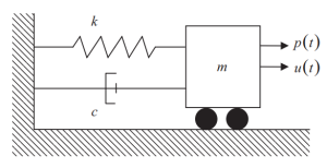
Φιγούρα 1. Ενιαίος βαθμός ελευθερίας (ΣΔΟΦ) Σύστημα. (γαβάθα, 2017, σελίδα 56)
Όλα τα στοιχεία πρέπει να ικανοποιούν τη συνθήκη δυναμικής ισορροπίας:
\({Μ}{\τελεία{εσύ}}+{ντο}{\τελεία{εσύ}}+{κ}{εσύ}={Π(τ)}\)
Αυτή είναι μια γραμμική διαφορική εξίσωση δεύτερης τάξης, και η λύση του έχει δύο συστατικά:
\({εσύ(τ)}={εσύ}_{η}(τ)+{εσύ}_{Π}(τ)\)
Οπου:
- \({εσύ(τ)}\) είναι η απόλυτη μετατόπιση.
- \({εσύ}_{η}(τ)\) είναι η ομοιογενής λύση, που αφορά γενικά την περίπτωση ελεύθερης δόνησης.
- \({εσύ}_{Π}(τ)\) είναι η συγκεκριμένη λύση σύμφωνα με τη διέγερση που εφαρμόζεται.
Θα εστιάσουμε μόνο στην ομοιογενή λύση για να περιγράψουμε τη συμπεριφορά των κραδασμών και τα πιο κρίσιμα δυναμικά χαρακτηριστικά που έχει μια κατασκευή.
Ας ορίσουμε τους παρακάτω όρους:
\({\ωμέγα_{ν}}={\τ.μ.(\frac {κ}{Μ})}\) Γωνιακή συχνότητα
\({\xi}={\frac{ντο}{{2}{Μ}{\ωμέγα_n}}}={\frac{ντο}{{2}{\τ.μ.(\frac {κ}{Μ})}}}\) Κλάσμα κρίσιμης απόσβεσης
Όταν το κλάσμα της κρίσιμης απόσβεσης είναι μικρότερο από 1, η θήκη δόνησης θα είναι υποαπόσβεση; αυτό είναι, θα ολοκληρωθούν κύκλοι πριν σταματήσει η κίνηση.
Η λύση είναι της ακόλουθης γενικής μορφής
\({u_h}={ε ^{{-\xi}{\ωμέγα_{ν}}{τ}}}{[{ΕΝΑ}{συν}{\ωμέγα_δ}{τ}+{σι}{χωρίς}{\ωμέγα_δ}{τ}]}\)
Οπου:
- Οι Α και Β είναι σταθερές ολοκλήρωσης που εξαρτώνται από τις αρχικές συνθήκες της κίνησης.
- \({\ωμέγα_δ}={\ωμέγα_n}{\τ.μ.({{1}-{\xi^2}})}\) είναι η αποσβεσμένη γωνιακή συχνότητα
Μόλις αξιολογηθούν οι σταθερές Α και Β, η γενική λύση για την θήκη χωρίς απόσβεση είναι
\({u_h}={ε ^{{-\xi}{\ωμέγα_{ν}}{τ}}}{[{u_0}{συν}{\ωμέγα_δ}{τ}+{\frac{{\τελεία{u_0}}+{\xi}{\ωμέγα_n}{u_0}}{\ωμέγα_δ}}{χωρίς}{\ωμέγα_δ}{τ}]}\)
Οπου:
- \({u_0}\) είναι η αρχική μετατόπιση μάζας
- \(\τελεία{u_0}\) είναι η αρχική ταχύτητα μάζας
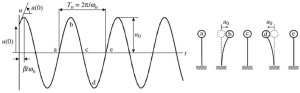
Αν σχεδιάσουμε τη λύση με κάποιες τιμές αρχικών συνθηκών, θα λάβουμε το παρακάτω σχήμα.
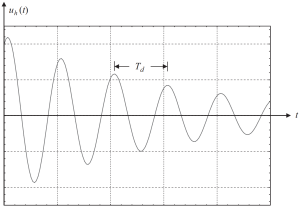
Φιγούρα 2. Η μετατόπιση έχει ως αποτέλεσμα ένα ομοιογενές τμήμα του διαλύματος σε μια υποκρίσιμη απόσβεση περίπτωση. (γαβάθα, 2017, σελίδα 58)
Στην άλλη περίπτωση, είναι σημαντικό να αναλύσουμε τι συμβαίνει όταν το κλάσμα της κρίσιμης απόσβεσης έχει μια τιμή 1. \({\xi}=1). Αυτή η συνθήκη συνεπάγεται μια δομή με πλήρη απόσβεση.
Η εξίσωση που πρέπει να χρησιμοποιήσετε είναι
\({u_h}={ε ^{{-\ωμέγα_{ν}}{τ}}}{\{u_0+({\τελεία{u_0}}+{\ωμέγα_n}{u_0}){τ}}\}\)
Και το γράφημά τους που δείχνει διαφορετικές περιπτώσεις αρχικών συνθηκών είναι στην παρακάτω εικόνα.
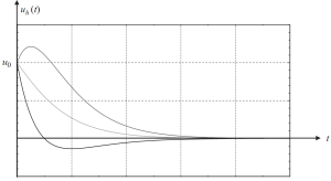
Φιγούρα 3. Η μετατόπιση οδηγεί σε ένα ομοιογενές τμήμα του διαλύματος σε μια κρίσιμη απόσβεση θήκη. (γαβάθα, 2017, σελίδα 58)
Παράμετροι απόκρισης
Η προηγούμενη ενότητα μας βοήθησε να ορίσουμε τη λύση για την ελεύθερη δυναμική δόνηση σε ένα σύστημα SDOF. Οι δύο κύριες παράμετροι είναι η φυσική συχνότητα \(\omega_n\) που δείχνει πώς η δομή θα δονείται από μόνη της, και το κλάσμα της κρίσιμης απόσβεσης \(\xi), που ορίζει την ταχύτητα στις δονήσεις αποσύνθεσης.
Γενικά, οι κατασκευές έχουν χαμηλή απόσβεση με μέγιστη τιμή \(\xi)=10 %. Εάν αξιολογήσουμε την αποσβεσμένη φυσική συχνότητα χρησιμοποιώντας αυτήν την τιμή, το αποτέλεσμα είναι \({\ωμέγα_δ}=0,995{\ωμέγα_n}\). Έτσι, συνιστάται η χρήση \({\ωμέγα_δ}{\πάχος περίπου}{\ωμέγα_n}\).
Μπορούμε να συνοψίσουμε τις δυναμικές ιδιότητες στον παρακάτω πίνακα.
| Γωνιακή συχνότητα (rad/s) | Φυσική συχνότητα (Ηζ) | Φυσική περίοδος (μικρό) | |
|---|---|---|---|
| Γωνιακή συχνότητα \({\ωμέγα_n}\) | \({\ωμέγα_n}\) | \(2{\πι}{f_n}\) | \(\frac{2{\πι}}{T_n}\) |
| Φυσική συχνότητα \({f_n}\) | \(\frac{\ωμέγα_n}{2{\πι}}\) | \(f_n\) | \(\frac{1}{T_n}\) |
| Φυσική περίοδος \({T_n}\) | \(\frac{2{\πι}}{\ωμέγα_n}\) | \(\frac{1}{f_n}\) | \(T_n\) |
Τραπέζι 1. Σχέση μεταξύ γωνιακής συχνότητας, φυσική συχνότητα, και περίοδος (γαβάθα, 2017, σελίδα 60)
Πολλαπλοί βαθμοί ελευθερίας
Όταν υπάρχουν πολλές μάζες σε μια δομή, πρέπει να ορίσουμε πολλαπλές συντεταγμένες για να περιγράψουμε τη θέση ανά πάσα στιγμή για αυτές τις μάζες. Ένα συγκεκριμένο και προφανές παράδειγμα φαίνεται στο παρακάτω σχήμα, που αποτελείται από ένα σύνθετο εκκρεμές όπου χρειάζονται διαφορετικές γωνίες για να καθοριστεί η θέση σε κάθε στιγμή κίνησης.
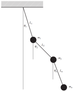
Φιγούρα 4. Εκκρεμές με πολλαπλές μάζες. (γαβάθα, 2017, σελίδα 53)
Σε ΑΥΤΗΝ την ΕΝΟΤΗΤΑ, αναλύουμε δομές’ γενική δυναμική απόκριση χρησιμοποιώντας την επέκταση των ιδιοτήτων ανάλυση συχνότητας για πολλαπλούς βαθμούς ελευθερίας.
Είναι επιτακτική ανάγκη να γνωρίζετε τη διαδικασία μοντελοποίησης όταν ασχολείστε με μια πραγματική δομή. Οι παρακάτω εικόνες περιγράφουν τα απαιτούμενα βήματα για την κατασκευή ενός μαθηματικού μοντέλου έτοιμου να εφαρμόσει την ανάλυση συχνότητας για να περιγράψει τη δυναμική του απόκριση.
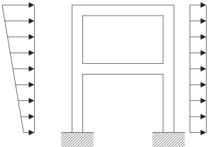
Φιγούρα 5. Φυσικό μοντέλο δομικού πλαισίου συνεχούς. (γαβάθα, 2017, σελίδα 23)
Το πρώτο βήμα περιλαμβάνει ομαδοποίηση μαζών σε κάθε επίπεδο διασταύρωση δοκών και υποστυλωμάτων. Κάθε κόμβος έχει τρεις πιθανές κινήσεις, δύο γραμμικές μετατοπίσεις, και μια περιστροφή. Να είμαστε συνεπείς στην ανάλυση, πρέπει να ληφθούν υπόψη οι μάζες και οι πολικές αδρανειακές ιδιότητες.
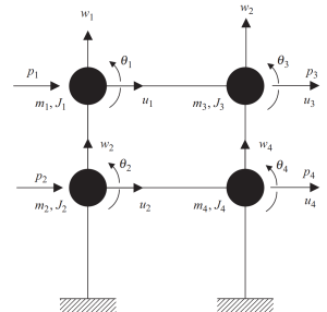
Φιγούρα 6. Συγκεντρωμένες μάζες σε κόμβους με βαθμούς ελευθερίας μετατόπισης και περιστροφής. Διακριτό Σύστημα. (γαβάθα, 2017, σελίδα 23)
Η μέθοδος στατικής συμπύκνωσης μπορεί να βοηθήσει στη μείωση της πολυπλοκότητας της ανάλυσης, παραβλέποντας την περιστροφική και μεταφορική αδράνεια.
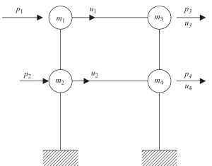
Φιγούρα 7. Στατική συμπύκνωση του βαθμού ελευθερίας μόνο σε οριζόντια μετατόπιση. (γαβάθα, 2017, σελίδα 23)
Στο τελευταίο βήμα, Μπορούμε να συγκεντρώσουμε σε δύο μόνο κόμβους την οριζόντια κίνηση για αυτό το παράδειγμα πλαισίου.
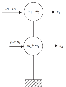
Φιγούρα 8. Τελική στατική συμπύκνωση σε δύο κόμβους και οριζόντια μετατόπιση βαθμός ελευθερίας. (γαβάθα, 2017, σελίδα 24)
Όπως κάναμε στην προηγούμενη ενότητα με το σύστημα SDOF, θα αναπτύξουμε τη λύση της εξίσωσης κίνησης για πολλαπλούς βαθμούς ελευθερίας.
Η εξίσωση κίνησης γράφει σε μορφή πίνακα ως
\([Μ]\{\τελεία{εσύ}\} + [ντο]\{\τελεία{εσύ}\}+[κ]\{u}={Π(τ)}\)
Οπου:
- \([Μ]\) είναι ο πίνακας μάζας
- \([ντο]\) είναι η μήτρα απόσβεσης του Coulumb
- \([κ]\) είναι το μήτρα ακαμψίας
Πρέπει να μελετήσουμε τη λύση ελεύθερης δόνησης για να λάβουμε τις παραμέτρους απόκρισης. Δεν ασκείται απόσβεση και δύναμη στο σύστημα, μόνο οι αρχικές συνθήκες που πρέπει να αξιολογηθούν.
\([Μ]\{\τελεία{εσύ}\} +[κ]\{u}={0}\)
Σε αναλογία με την πρώτη περίπτωση για ΣΔΟΦ, μπορούμε να δοκιμάσουμε ένα ημιτονοειδές διάλυμα της μορφής.
\({εσύ(τ)}={\phi}{({ένα}{συν}{\ωμέγα}{τ}+{σι}{χωρίς}{\ωμέγα}{τ})}\)
\({\τελεία{εσύ}{(τ)}}={-{\ωμέγα}^ 2}{\phi}{({ένα}{συν}{\ωμέγα}{τ}+{σι}{χωρίς}{\ωμέγα}{τ})}\)
Στο οποίο το διάνυσμα \(\φι) είναι ένα διάνυσμα σχήματος που δεν εξαρτάται από το χρόνο. Οι συντελεστές “ένα” και “σι” είναι σταθερές που λαμβάνονται κατά την αξιολόγηση των αρχικών συνθηκών.
Αφού αντικατασταθούν και οι δύο εκφράσεις για τη δοκιμαστική λύση στην εξίσωση κίνησης, λαμβάνουμε το γραμμικό πρόβλημα ιδιοτιμής-ιδιοδιάνυσμα:
\([κ]{\phi}={{\ωμέγα}^ 2}[Μ]{\phi}\)
Οπου:
- \({{\ωμέγα}^ 2}\) είναι το σύνολο των ιδιοτιμών
- \({\phi}\) είναι το σύνολο των ιδιοδιανυσμάτων
Η λύση σε αυτό το κλασικό πρόβλημα για το παράδειγμα πλαισίου στα πιο πρόσφατα σχήματα δείχνει πώς θα δονούνται οι μάζες. Αυτό σημαίνει ότι κάθε μάζα θα κινείται σε οριζόντια κατεύθυνση σύμφωνα με την τιμή των ιδιοδιανυσμάτων.
Κοιτάξτε την παρακάτω εικόνα αυτής της συμπεριφοράς.
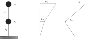
Εικόνα Νο.9. Ανάλυση συχνότητας που δείχνει τα αποτελέσματα των δύο ιδιοδιανυσμάτων. (γαβάθα, 2017, Σελίδα 135)
SkyCiv Structural 3D
Εκτελέστε ανάλυση συχνότητας για τις δομές σας με SkyCiv Structural 3D. Εγγραφείτε σήμερα για να ξεκινήσετε!
βιβλιογραφικές αναφορές:
- Εντουάρντο Καουζέλ, (2017). “Προηγμένη Δυναμική Δομής” 1η έκδοση, Cambridge University Press