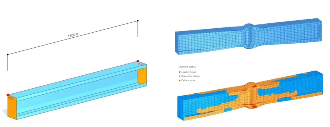
Σε αυτό το παράδειγμα, θα δείξουμε πώς να αναλύσουμε ένα μέλος κατασκευασμένο από ένα λεπτό προφίλ χαλύβδινης πλάκας. Το προφίλ έχει το τμήμα καναλιού με πάχος πλάκας 1.5 χιλ. και μήκος του 1500 χιλ. Διαφράγματα, με πάχος 20 χιλ, συνδέονται και στα δύο άκρα του μέλους. Οι οριακές συνθήκες εφαρμόζονται στα άκρα του μέλους: η αριστερή πλευρά τυλίγεται σε ρολό ενώ το αντίθετο άκρο είναι καρφιτσωμένο. Οι ιδιότητες του υλικού για τα εξαρτήματα καθορίζονται με αντοχή διαρροής (κηλίδα) του 355 MPa. Το μέλος υπόκειται σε αξονική θλιπτική δύναμη ίση με 1000 ΚΝ.
Για να δείτε αυτή την ανάλυση στην πράξη και να κατανοήσετε καλύτερα, παρακολουθήστε τη γρήγορη επίδειξη βίντεο που παρέχεται παρακάτω:
Βήμα 1. Μοντέλα μέρη
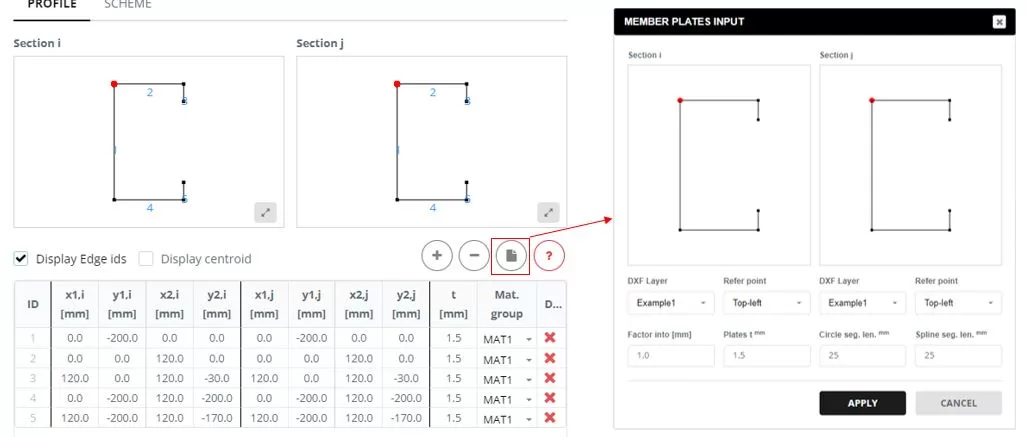
Μεταβείτε στα «κύρια μέρη’ μενού και επιλέξτε το προφίλ '’ αυτί. Εισαγάγετε τις άκρες και για την εκκίνηση (Εγώ) και τελειώνει (ι) τμήματα. Για να εισαγάγετε τα τμήματα’ γεωμετρία, μπορείτε να εισαγάγετε ένα αρχείο DXF που είναι αποθηκευμένο τοπικά στον υπολογιστή σας. Το αρχείο DXF μπορεί να ληφθεί από εδώ
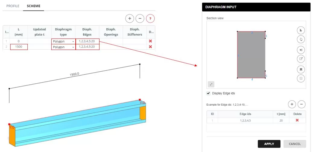
Μεταβείτε στο «ΣΧΕΔΙΟ’ αυτί. Ορίστε το μήκος μέλους σε 1500 χιλ. Προσθέστε διαφράγματα στα άκρα, Επιλέγοντας το «πολύγωνο’ τύπος. Οι άκρες για το διάφραγμα ορίζονται σε ένα αναδυόμενο παράθυρο που εμφανίζεται όταν κάνετε κλικ στις ακμές του διαφράγματος’ κελί στήλης. Στην «είσοδο του διαφράγματος», Επιλέξτε τις άκρες που σχηματίζουν το σχήμα του διαφράγματος και εισάγετε το πάχος (τ).
Βήμα 2. Πλέγμα
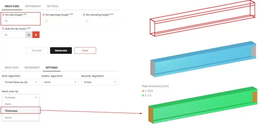
Πλοηγηθείτε στο 'Meshing’ μενού. Ρυθμίστε το μέγεθος του στοιχείου FE σε 15 χιλ, Στη συνέχεια, κάντε κλικ στο "Δημιουργία’ κουμπί. Το χρώμα του πλέγματος μπορεί να ενημερωθεί ανάλογα με το πάχος της πλάκας ("ΡΥΘΜΙΣΕΙΣ" > ‘Mesh color by’)
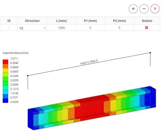
Βήμα 3. Ατέλειες
Πλοηγηθείτε στο «Ατέλεια’ μενού. Ορίστε τις ρυθμίσεις, μετά κάντε κλικ στην Προεπισκόπηση’ κουμπί.
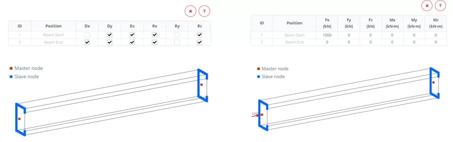
Βήμα 4. Όρια και φορτίο
Μεταβείτε στα «όρια» > Μενού «άκαμπτα άκρα». Ρυθμίστε τους περιορισμούς του τελικού ορίου. Μεταβείτε στα «φορτία» > Μενού «άκαμπτα άκρα». Εφαρμόστε ένα αξονικό φορτίο 1000 KN στο αριστερό άκρο του μέλους για συμπίεση.
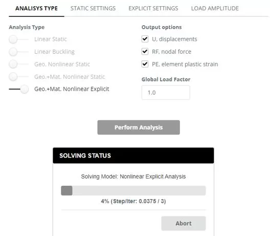
Βήμα 5. Ανάλυση και παρακολούθηση μετατόπισης φορτίου
Μεταβείτε στο μενού 'Ανάλυση'. Επιλέξτε μη γραμμική ρητή συμπεριλαμβανομένης της γεωμετρίας και της μη γραμμικότητας υλικού. Κάντε κλικ στο κουμπί "Εκτέλεση ανάλυσης".
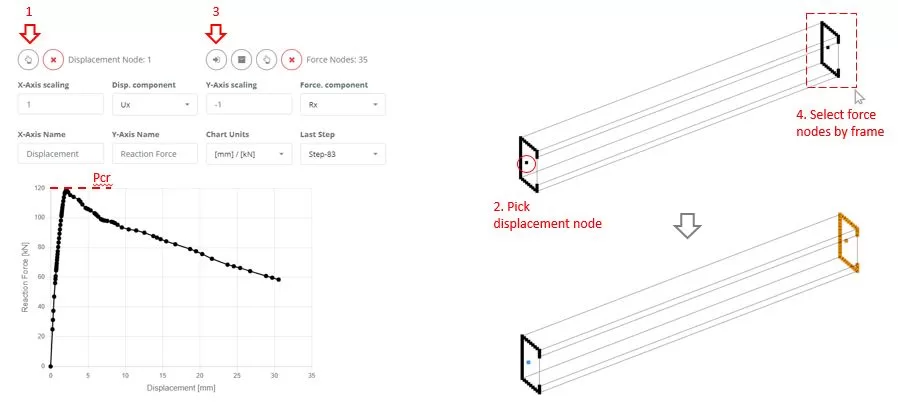
Ενώ η ανάλυση βρίσκεται σε εξέλιξη, Πλοηγηθείτε στο μενού "Χάρτης". Πρώτα, Επιλέξτε έναν κόμβο για να μετρήσετε την μετατόπιση UX (βήματα 1 και 2). Τότε, Χρήση επιλογής πλαισίου, Επιλέξτε κόμβους από τους οποίους μπορείτε να εξαγάγετε τις δυνάμεις αντίδρασης RX (βήματα 3 και 4). Παρακολουθήστε τις αλλαγές του χάρτη για να προσδιορίσετε την κρίσιμη δύναμη (PCR) που οδηγεί τη δομή σε αποτυχία. Τερματίστε τη συνεχιζόμενη ανάλυση μόλις ανιχνευθεί η κατάσταση αποτυχίας.
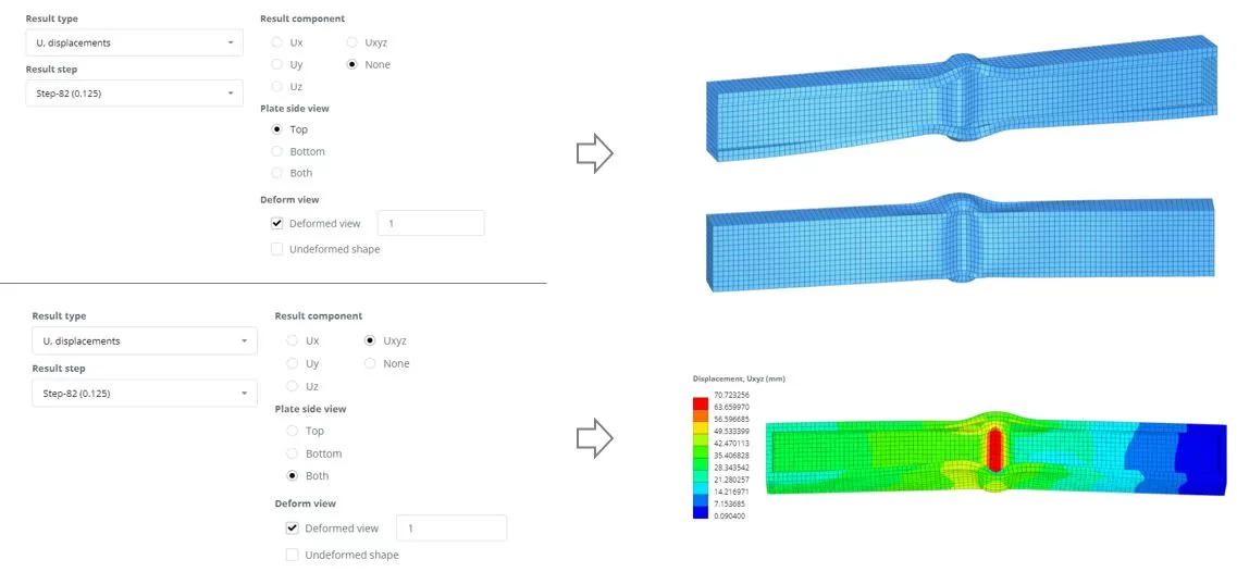
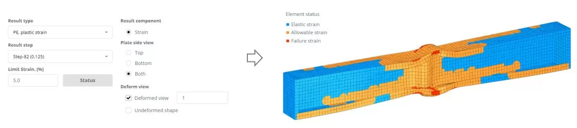
Βήμα 6. Αποτελέσματα
Μεταβείτε στα «αποτελέσματα»’ μενού, Επιλέξτε τις προτιμώμενες επιλογές αποτελεσμάτων σας, και κάντε κλικ στην επιλογή "Εμφάνιση’ Για να δείτε την παραμορφωμένη κατάσταση του μοντέλου.
Λογισμικό δομικής μηχανικής SkyCiv
Αν δεν το έχετε κάνει ήδη, εγγραφείτε δωρεάν με το SkyCiv σήμερα και ξεκλειδώστε ισχυρά εργαλεία δομικής ανάλυσης και σχεδίασης για να επιταχύνετε τα μηχανολογικά σας έργα!