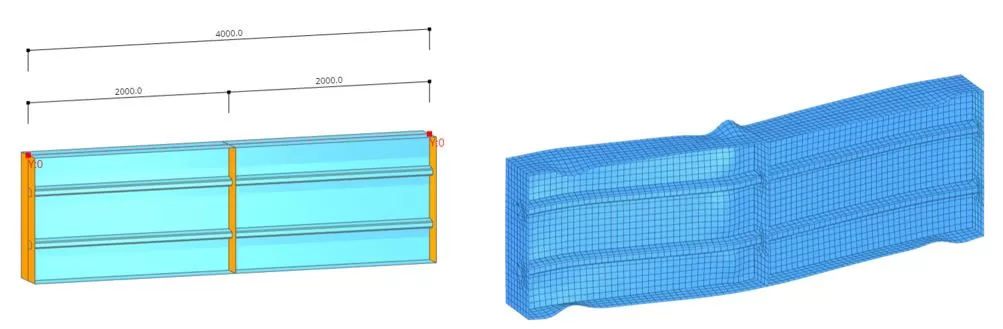
Σε αυτό το παράδειγμα, Θα δείξουμε πώς να αναλύσουμε μια δέσμη που σκληρύνει με οριζόντια και κατακόρυφα στοιχεία και υποβάλλονται σε αξονικές και διατμητικές δυνάμεις. Η δέσμη έχει μήκος 4000 mm και ενισχύεται με δύο οριζόντιες ενισχυτές που έχουν κλειστό τμήμα, καθώς και τρεις κατακόρυφες ενισχυτές. Οι φλάντζες πάνω και κάτω έχουν πάχος 16 χιλ, Ο ιστός είναι 10 πάχος mm, Οι διαμήκεις νευρώσεις είναι 5 πάχος mm, Και οι κατακόρυφες ενισχύσεις είναι 15 πάχος mm. Τα άκρα της δέσμης έχουν ρυθμιστεί με κυλιόμενες και καρφωμένες οριακές συνθήκες. Η δέσμη υποβλήθηκε σε αξονικό φορτίο 15000 δυνάμεις kn και διάτμησης του 2000 ΚΝ. Τα υλικά έχουν δύναμη απόδοσης (κηλίδα) του 355 MPa.

Η επερχόμενη ανάλυση θα περιλαμβάνει τόσο τη γεωμετρική όσο και τη μη γραμμικότητα του υλικού. Προσφέρει επίσης παρακολούθηση σε πραγματικό χρόνο της καμπύλης μετατόπισης φορτίου, επιτρέποντας μια εμπεριστατωμένη διερεύνηση της χωρητικότητας του μέλους κατά τη βελτιστοποίηση του υπολογιστικού χρόνου. Τα αποτελέσματα θα παρέχουν πληροφορίες για την ικανότητα του μέλους, η παραμορφωμένη του κατάσταση, και την κατάσταση αποτυχίας του.

Βήμα 1. Μοντέλα μέρη

Μεταβείτε στα «κύρια μέρη’ μενού και επιλέξτε το προφίλ '’ αυτί. Για να εισαγάγετε τα τμήματα’ γεωμετρία, Εισαγάγετε ένα αρχείο DXF που είναι αποθηκευμένο τοπικά στον υπολογιστή σας. Το αρχείο DXF μπορεί να ληφθεί από εδώ

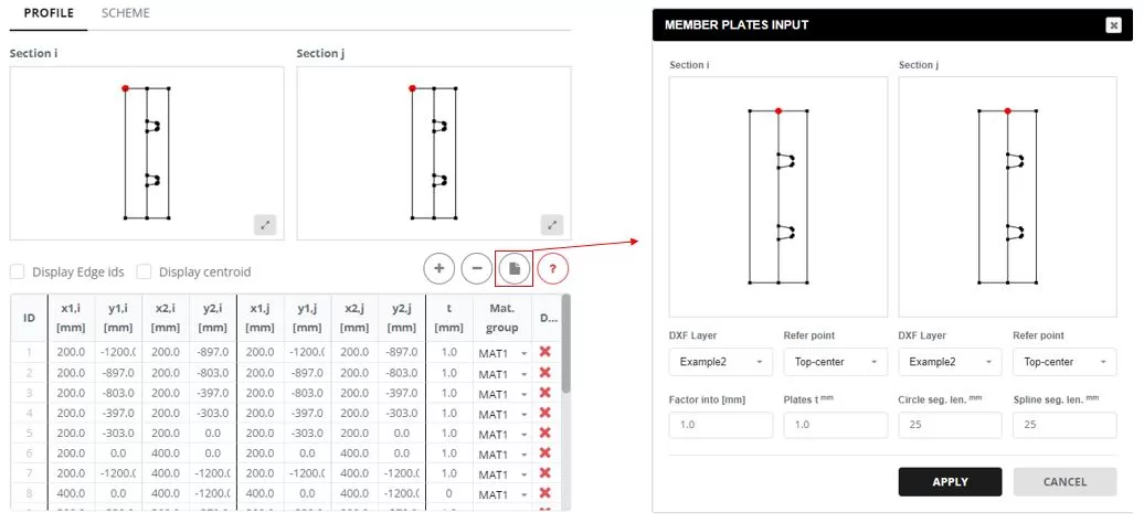
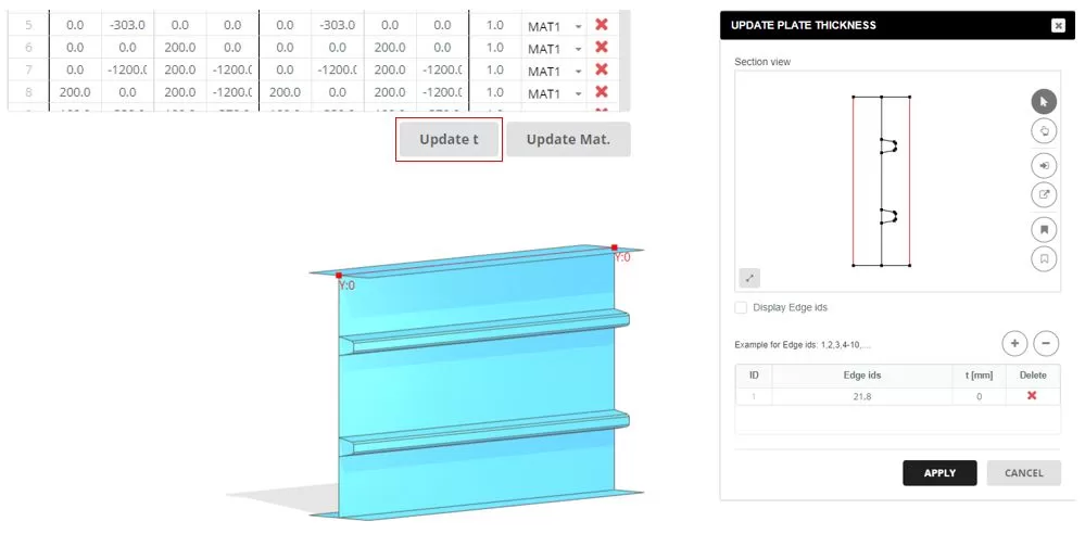
Κάντε κλικ στο κουμπί "Ενημέρωση t". Επιλέξτε πλευρικές άκρες (21,8) και ρυθμίστε το πάχος (τ) προς το 0 χιλ.

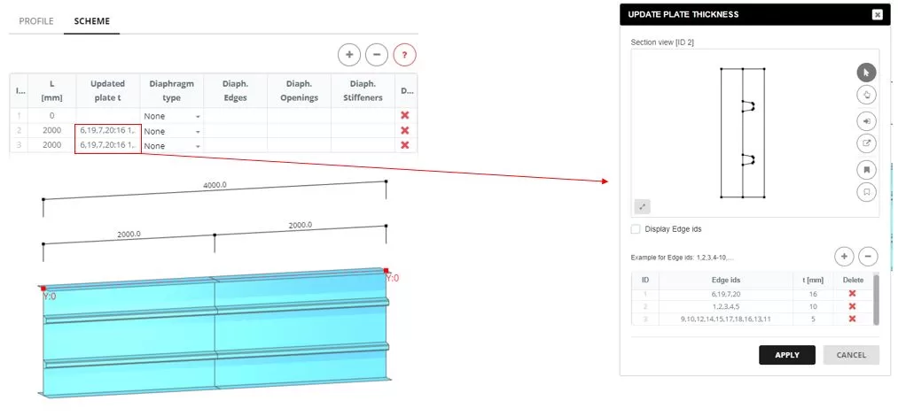
Μεταβείτε στο πρόγραμμα '’ αυτί. Διαμορφώστε δύο τμήματα, Ρύθμιση του μήκους του καθενός 2000 χιλ. Όταν κάνετε κλικ στην «ενημερωμένη πλάκα t’ κελί στήλης, Θα εμφανιστεί ένα αναδυόμενο παράθυρο. Σε αυτό το παράθυρο, Ενημερώστε το πάχος για τις άκρες κάθε τμήματος: Ρυθμίστε τις κορυφαίες φλάντζες στο T = 16 mm, ο ιστός σε t = 10 mm, και νευρώσεις σε t = 5 mm.

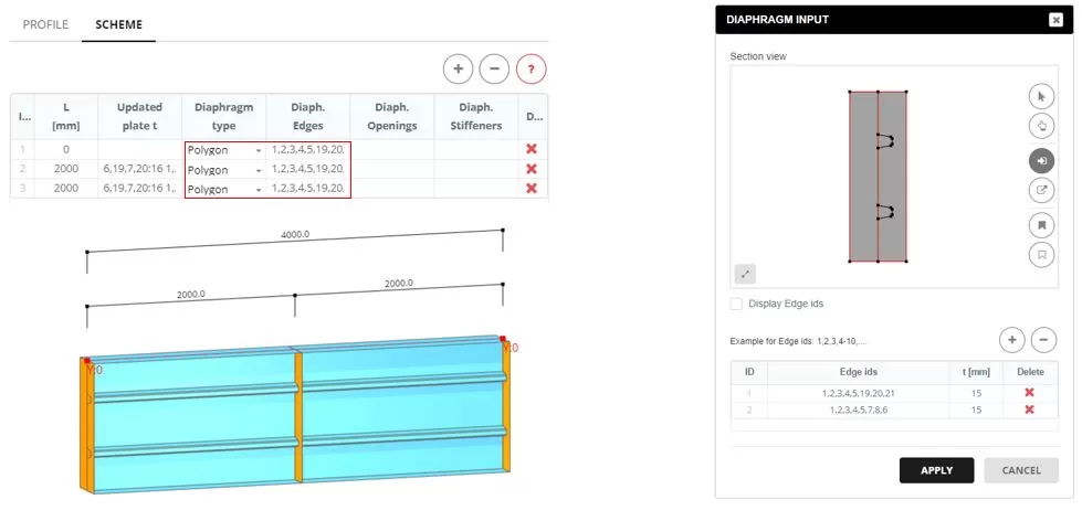
Προσθέστε διαφράγματα στα τμήματα, Επιλέγοντας το «πολύγωνο’ τύπος. Οι άκρες για το διάφραγμα ορίζονται σε ένα αναδυόμενο παράθυρο που εμφανίζεται όταν κάνετε κλικ στις ακμές του διαφράγματος’ κελί στήλης. Στην «είσοδο του διαφράγματος», Επιλέξτε τις άκρες που σχηματίζουν το σχήμα του διαφράγματος και εισάγετε το πάχος (τ).

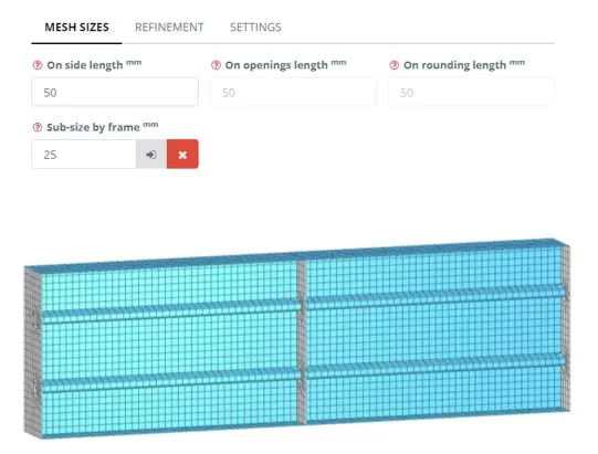
Βήμα 2. Πλέγμα

Πλοηγηθείτε στο 'Meshing’ μενού. Ρυθμίστε το μέγεθος του στοιχείου FE σε 50 χιλ, Στη συνέχεια, κάντε κλικ στο "Δημιουργία’ κουμπί.

Βήμα 3. Όρια και φορτίο

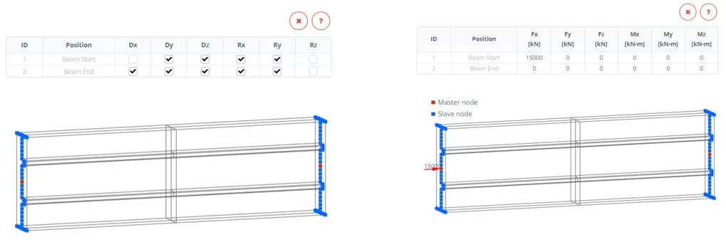
Μεταβείτε στα «όρια» > Μενού «άκαμπτα άκρα». Ρυθμίστε τους περιορισμούς του τελικού ορίου. Μεταβείτε στα «φορτία» > Μενού «άκαμπτα άκρα». Εφαρμόστε ένα αξονικό φορτίο 15000 KN στο αριστερό άκρο του μέλους για συμπίεση.

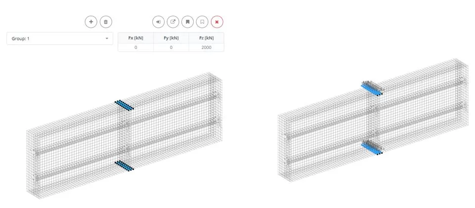
Μεταβείτε στα «φορτία > «Δύναμη (Εθιμο)«Μενού. Προσθέστε μια νέα ομάδα φορτίου με την ονομασία 'Group: 1''. Επιλέξτε τα στοιχεία τόσο παραπάνω όσο και κάτω από το κεντρικό κατακόρυφο ενισχυτικό, και στη συνέχεια να εκχωρήσετε ένα φορτίο διάτμησης FZ του 2000 ΚΝ

Βήμα 4. Ανάλυση και παρακολούθηση μετατόπισης φορτίου

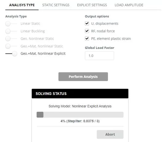
Μεταβείτε στο μενού 'Ανάλυση'. Επιλέξτε μη γραμμική ρητή συμπεριλαμβανομένης της γεωμετρίας και της μη γραμμικότητας υλικού. Κάντε κλικ στο κουμπί "Εκτέλεση ανάλυσης".

 

 

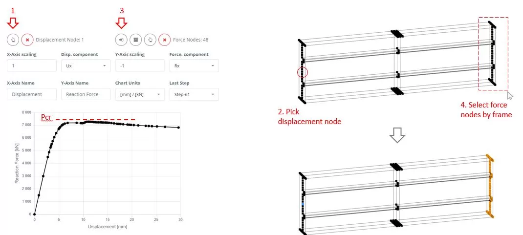
Ενώ η ανάλυση βρίσκεται σε εξέλιξη, Πλοηγηθείτε στο μενού "Χάρτης". Πρώτα, Επιλέξτε έναν κόμβο για να μετρήσετε την μετατόπιση UX (βήματα 1 και 2). Τότε, Χρήση επιλογής πλαισίου, Επιλέξτε κόμβους από τους οποίους μπορείτε να εξαγάγετε τις δυνάμεις αντίδρασης RX (βήματα 3 και 4). Παρακολουθήστε τις αλλαγές του χάρτη για να προσδιορίσετε την κρίσιμη δύναμη (PCR) που οδηγεί τη δομή σε αποτυχία. Τερματίστε τη συνεχιζόμενη ανάλυση μόλις ανιχνευθεί η κατάσταση αποτυχίας.

 

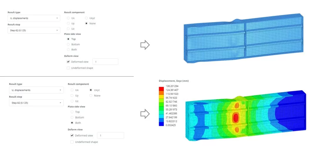
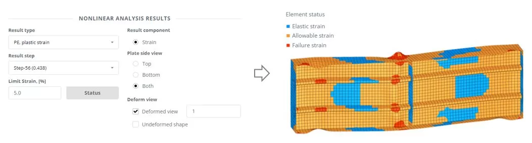
Βήμα 5. Αποτελέσματα

Μεταβείτε στα «αποτελέσματα»’ μενού, Επιλέξτε τις προτιμώμενες επιλογές αποτελεσμάτων σας, και κάντε κλικ στην επιλογή "Εμφάνιση’ Για να δείτε την παραμορφωμένη κατάσταση του μοντέλου.