Basisplatten -Designbeispiel unter Verwendung von AISC 360-22 und ACI 318-19
Problemanweisung
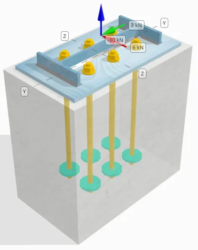
Stellen Sie fest, ob die geplante Verbindung zwischen Säule und Grundplatte ausreichend ist 30 kN Zugbelastung, 3 kN Vy Scherlast, und 6 kN Vz Querlast.
Gegebene Daten
Spalte:
Spaltenabschnitt: B14x30
Säulenbereich: 5709.7 mm2
Säulenmaterial: A992
Grundplatte:
Grundplattenabmessungen: 250 mmx 250 mm
Grundplattendicke: 12 mm
Grundplattenmaterial: A992
Fugenmörtel:
Fugendicke: 0 mm
Beton:
Konkrete Abmessungen: 300 mmx 500 mm
Betondicke: 500 mm
Betonmaterial: 20.7 MPa
Geknackt oder ungekrönt: Geknackt
Anker:
Ankerdurchmesser: 16 mm
Effektive Einbettungslänge: 400 mm
Ankerende: Kreisförmige Platte
Eingebetteter Plattendurchmesser: 70 mm
Dicke eingebetteter Platten: 10 mm
Stahlmaterial: F1554 Gr.55
Gewinde in der Scherebene: Im Lieferumfang enthalten
Schweißnähte:
Schweißnahtgröße: 7 mm
Füllmetallklassifizierung: E70XX
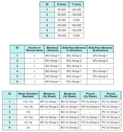
Ankerdaten (von Skyciv -Taschenrechner):
Modell im kostenlosen SkyCiv-Tool
Modellieren Sie noch heute das oben stehende Grundplattendesign mit unserem kostenlosen Online-Tool! Keine Anmeldung erforderlich.
Hinweis
Der Zweck dieses Konstruktionsbeispiels besteht darin, die schrittweisen Berechnungen für Kapazitätsnachweise bei gleichzeitiger Scher- und Axiallast zu demonstrieren. Einige der erforderlichen Prüfungen wurden bereits in den vorherigen Entwurfsbeispielen besprochen. Bitte beachten Sie die in den einzelnen Abschnitten bereitgestellten Links.
Schritt-für-Schritt-Berechnungen
Prüfen #1: Berechnen Sie die Schweißkapazität
Zur Bestimmung der Schweißleistung bei gleichzeitiger Belastung, Wir müssen zunächst den Schweißbedarf aufgrund der berechnen Scherbelastung und der Schweißbedarf aufgrund der Zugbelastung. Sie können sich darauf beziehen link für das Verfahren zur Ermittlung der Schweißnahtanforderungen für Scherung, und das link für die Anforderungen beim Zugschweißen.
Für dieses Design, bleibt die Schweißbedarf an der Bahn aufgrund der Zugbelastung ergibt sich folgendes Ergebnis, wobei die Belastung ausgedrückt wird als Kraft pro Längeneinheit.
\(r_{u,\Text{Netz}} = frac{T_{u,\Text{Anker}}}{l_{\Text{eff}}} = frac{5\ \Text{kN}}{93.142\ \Text{mm}} = 0.053681\ \Text{kN / mm}\)
Außerdem, bleibt die Schweißspannung an jedem Teil des Säulenabschnitts aufgrund der Scherbelastung wird bestimmt als:
\(v_{ui} = frac{V_y}{L_{\Text{schweißen}}} = frac{3\ \Text{kN}}{1250.7\ \Text{mm}} = 0.0023987\ \Text{kN / mm}\)
\(v_{Zu} = frac{V_z}{L_{\Text{schweißen}}} = frac{6\ \Text{kN}}{1250.7\ \Text{mm}} = 0.0047973\ \Text{kN / mm}\)
Da es eine Kombination aus Zug- und Scherbelastungen gibt Netz, Wir müssen das Resultierende erhalten. Dies wird als Kraft pro Längeneinheit ausgedrückt, wir haben:
\(r_u = sqrt{(r_{u,\Text{Netz}})^ 2 + (v_{ui})^ 2 + (v_{Zu})^ 2}\)
\(r_u = sqrt{(0.053681\ \Text{kN / mm})^ 2 + (0.0023987\ \Text{kN / mm})^ 2 + (0.0047973\ \Text{kN / mm})^ 2}\)
\(r_u = 0.053949\ \Text{kN / mm}\)
Für die Flansche, Es liegen nur Schubspannungen vor. So, das Ergebnis ist:
\(r_u = sqrt{(v_{ui})^ 2 + (v_{Zu})^ 2}\)
\(r_u = sqrt{(0.0023987\ \Text{kN / mm})^ 2 + (0.0047973\ \Text{kN / mm})^ 2} = 0.0053636\ \Text{kN / mm}\)
Als nächstes, wir berechnen die Schweißkapazitäten. Für den Flansch, Wir bestimmen den Winkel θ Verwendung der Vz und Vy Ladungen.
\( \Theta = tan^{-1}\!\links(\frac{v_{ui}}{v_{Zu}}\richtig) = tan^{-1}\!\links(\frac{0.0023987\ \Text{kN / mm}}{0.0047973\ \Text{kN / mm}}\richtig) = 0.46365\ \Text{Arbeit} \)
Folglich, bleibt die kds Faktor und Schweißkapazität werden mit berechnet AISC 360-22 Gl. J2-5 und Gl. J2-4.
\(k_{ds} = 1.0 + 0.5(\ohne(\theta))^{1.5} = 1 + 0.5 \mal (\ohne(0.46365\ \Text{Arbeit}))^{1.5} = 1.1495\)
\(\PHI R_{n,flg} = phi,0,6,F_{Exx}\,E_w,k_{ds} = 0.75 \mal 0.6 \mal 480\ \Text{MPa} \mal 4.95\ \Text{mm} \mal 1.1495 = 1.2291\ \Text{kN / mm}\)
Für das Web, Wir berechnen den Winkel θ mit einer anderen Formel. Beachten Sie, dass Wow wird in der Formel verwendet, da es die Last parallel zur Schweißachse darstellt.
\( \Theta = cos^{-1}\!\links(\frac{v_{ui}}{r_u}\richtig) = cos^{-1}\!\links(\frac{0.0023987\ \Text{kN / mm}}{0.053949\ \Text{kN / mm}}\richtig) = 1.5263\ \Text{Arbeit} \)
Verwenden von AISC 360-22 Gl. J2-5 und Gl. J2-4, bleibt die kds Der Schweißfaktor und die daraus resultierende Schweißkapazität werden auf die gleiche Weise ermittelt.
\(k_{ds} = 1.0 + 0.5(\ohne(\theta))^{1.5} = 1 + 0.5 \mal (\ohne(1.5263\ \Text{Arbeit}))^{1.5} = 1.4993\)
\(\PHI R_{n,Netz} = phi,0,6,F_{Exx}\,E_w,k_{ds} = 0.75 \mal 0.6 \mal 480\ \Text{MPa} \mal 4.95\ \Text{mm} \mal 1.4993 = 1.603\ \Text{kN / mm}\)
zuletzt, wir treten auf unedle Metallschecks sowohl für die Säule als auch für die Grundplatte, Ermitteln Sie dann die maßgebliche Basismetallkapazität.
\( \PHI R_{nbm,col} = phi,0,6,F_{u,col}\,t_{col,Hälfte} = 0.75 \mal 0.6 \mal 448.2\ \Text{MPa} \mal 3.429\ \Text{mm} = 0.6916\ \Text{kN / mm} \)
\( \PHI R_{nbm,bp} = phi,0,6,F_{u,bp}\,t_{bp} = 0.75 \mal 0.6 \mal 400\ \Text{MPa} \mal 12\ \Text{mm} = 2.1595\ \Text{kN / mm} \)
\( \PHI R_{nbm} = minbig(\PHI R_{nbm,bp},\ \PHI R_{nbm,col}\groß) = min(2.1595\ \Text{kN / mm},\ 0.6916\ \Text{kN / mm}) = 0.6916\ \Text{kN / mm} \)
Wir vergleichen dann die Kehlnahtkapazitäten und Basismetallkapazitäten für die Schweißanforderungen an der Flansche und Steg getrennt.
Schon seit 0.053949 kN / mm < 0.6916 kN / mm, Die Schweißkapazität ist ausreichend.
Prüfen #2: Berechnen Sie die Kapazität der Grundplattenflexus aufgrund der Spannungsbelastung
Ein Designbeispiel für die Biegenachgiebigkeit der Grundplatte wurde bereits im Grundplatten-Designbeispiel für Spannung besprochen. Die Schritt-für-Schritt-Berechnung finden Sie unter diesem Link.
Prüfen #3: Berechnen Sie die Ankerstange Zugkapazität
Ein Bemessungsbeispiel für die Zugfähigkeit der Ankerstange wird bereits im Grundplatten-Bemessungsbeispiel für Spannung besprochen. Die Schritt-für-Schritt-Berechnung finden Sie unter diesem Link. Die Schritt-für-Schritt-Berechnung finden Sie unter diesem Link.
Prüfen #4: Berechnen Sie die Betonausbruchkapazität in der Spannung
Ein Entwurfsbeispiel für die Fähigkeit des Betons, unter Spannung auszubrechen, wurde bereits im Grundplatten-Entwurfsbeispiel für Spannung besprochen. Die Schritt-für-Schritt-Berechnung finden Sie unter diesem Link. Die Schritt-für-Schritt-Berechnung finden Sie unter diesem Link.
Prüfen #5: Berechnen Sie die Ankerauszugskapazität
Ein Entwurfsbeispiel für die Ankerauszugskapazität wurde bereits im Grundplatten-Entwurfsbeispiel für Spannung besprochen. Die Schritt-für-Schritt-Berechnung finden Sie unter diesem Link. Die Schritt-für-Schritt-Berechnung finden Sie unter diesem Link.
Prüfen #6: Berechnen Sie die Biegekapazität der Einbettplatte
Ein Entwurfsbeispiel für den ergänzenden Nachweis der Biegestreckfähigkeit der eingebetteten Platte wird bereits im Entwurfsbeispiel der Grundplatte für Spannung besprochen. Die Schritt-für-Schritt-Berechnung finden Sie unter diesem Link.
Prüfen #7: Berechnen Sie die Blowout-Kapazität der Seitengesicht in der y-Richtung
Zur Berechnung der Side-Face-Blowout (SFBO) Kapazität, Wir ermitteln zunächst die Summe Spannungskraft auf den Ankern, die der Kante am nächsten liegen. Für diesen Check, Wir werden die Kapazität der Kante entlang bewerten Y-Richtung.
Da sich die Ausfallkegelprojektionen des SFBO entlang der Y-Richtung überlappen, Die Anker werden als behandelt Ankergruppe.
Der Gesamtspannungsbedarf der Ankergruppe wird berechnet als::
\(N_{Tun} = left(\frac{N_x}{N_{ein,t}}\richtig) N_{j,G1} = left(\frac{30\ \Text{kN}}{6}\richtig) \mal 3 = 15\ \Text{kN}\)
Als nächstes, Wir bestimmen die Randabstände:
\(c_{mit,\Min.} = min(c_{\Text{links},G1},\ c_{\Text{richtig},G1}) = min(100\ \Text{mm},\ 200\ \Text{mm}) = 100\ \Text{mm}\)
\(c_{j,\Min.} = min(c_{\Text{oben},G1},\ c_{\Text{Unterseite},G1}) = min(150\ \Text{mm},\ 150\ \Text{mm}) = 150\ \Text{mm}\)
Verwendung dieser Randabstände, wir berechnen die Kapazität der Ankergruppe in Übereinstimmung mit ACI 318-19 Gl. (17.6.4.1).
\(N_{als} = left(\frac{1 + \dfrac{c_{j,\Min.}}{c_{mit,\Min.}}}{4} + \frac{S_{Summe,j,G1}}{6\,c_{mit,\Min.}}\richtig)\mal 13 \mal links(\frac{c_{mit,\Min.}}{1\ \Text{mm}}\richtig)\mal sqrt{\frac{EIN_{brg}}{\Text{mm}^ 2}}\ \lambda_a sqrt{\frac{f_c}{\Text{MPa}}}\mal 0.001\ \Text{kN}\)
\(N_{als} = left(\frac{1 + \dfrac{150\ \Text{mm}}{100\ \Text{mm}}}{4} + \frac{200\ \Text{mm}}{6\mal 100\ \Text{mm}}\richtig)\mal 13 \mal links(\frac{100\ \Text{mm}}{1\ \Text{mm}}\richtig)\mal sqrt{\frac{3647.4\ \Text{mm}^ 2}{1\ \Text{mm}^ 2}}\mal 1 \mal sqrt{\frac{20.68\ \Text{MPa}}{1\ \Text{MPa}}}\mal 0.001\ \Text{kN}\)
\(N_{als} = 342.16\ \Text{kN}\)
In der ursprünglichen Gleichung, Ein Reduktionsfaktor wird angewendet, wenn der Ankerabstand kleiner ist als 6ca₁, Vorausgesetzt, die Kopfanker haben einen ausreichenden Randabstand. Jedoch, in diesem Designbeispiel, schon seit ca₂ < 3ca₁, Der SkyCiv-Rechner wendet einen zusätzlichen Reduktionsfaktor an, um die reduzierte Kantenkapazität zu berücksichtigen.
Schließlich, bleibt die Auslegung der SFBO-Kapazität ist:
\(\phi N_{als} = phi,N_{als} = 0.7 \mal 342.16\ \Text{kN} = 239.51\ \Text{kN}\)
Schon seit 15 kN < 239.51 kN, Die SFBO-Kapazität entlang der Y-Richtung beträgt ausreichend.
Prüfen #8: Berechnen Sie die Blowout-Kapazität der Seitengesicht in der Z-Richtung
Nach dem gleichen Ansatz wie in Prüfen #7, der Gesamtspannungsbedarf der Ankergruppe für die Anker, die am nächsten liegen Z-Richtung Kante ist:
\(N_{Tun} = left(\frac{N_x}{N_{ein,t}}\richtig)N_{mit,G1} = left(\frac{30\ \Text{kN}}{6}\richtig)\mal 2 = 10\ \Text{kN}\)
Mit der Randabstände werden berechnet als:
\(c_{j,\Min.} = min(c_{\Text{oben},G1},\ c_{\Text{Unterseite},G1}) = min(150\ \Text{mm},\ 350\ \Text{mm}) = 150\ \Text{mm}\)
\(c_{mit,\Min.} = min(c_{\Text{links},G1},\ c_{\Text{richtig},G1}) = min(100\ \Text{mm},\ 100\ \Text{mm}) = 100\ \Text{mm}\)
Mit der nominale SFBO-Kapazität wird dann bestimmt als:
\(N_{als} = left(\frac{1 + \dfrac{c_{mit,\Min.}}{c_{j,\Min.}}}{4} + \frac{S_{Summe,mit,G1}}{6\,c_{j,\Min.}}\richtig)\mal 13 \mal links(\frac{c_{j,\Min.}}{1\ \Text{mm}}\richtig)\mal sqrt{\frac{EIN_{brg}}{\Text{mm}^ 2}}\ \lambda_a sqrt{\frac{f_c}{\Text{MPa}}}\mal 0.001\ \Text{kN}\)
\(N_{als} = left(\frac{1 + \dfrac{100\ \Text{mm}}{150\ \Text{mm}}}{4} + \frac{100\ \Text{mm}}{6\mal 150\ \Text{mm}}\richtig)\mal 13 \mal links(\frac{150\ \Text{mm}}{1\ \Text{mm}}\richtig)\mal sqrt{\frac{3647.4\ \Text{mm}^ 2}{1\ \Text{mm}^ 2}}\mal 1 \mal sqrt{\frac{20.68\ \Text{MPa}}{1\ \Text{MPa}}}\mal 0.001\ \Text{kN}\)
\(N_{als} = 282.65\ \Text{kN}\)
Da der Randabstand ca₂ ist immer noch weniger als 3ca₁, Es wird der gleiche modifizierte Reduktionsfaktor angewendet.
Schließlich, bleibt die Auslegung der SFBO-Kapazität ist:
\(\phi N_{als} = phi,N_{als} = 0.7 \mal 282.65\ \Text{kN} = 197.86\ \Text{kN}\)
Schon seit 10 kN < 197.86 kN, die SFBO-Kapazität entlang der Z-Richtung ist ausreichend.
Prüfen #9: Berechnen Sie die Breakout-Kapazität (Vy Schere)
Ein Entwurfsbeispiel für die Betonausbrechkapazität bei Vy-Scherung wird bereits im Grundplatten-Entwurfsbeispiel für Scherung besprochen. Die Schritt-für-Schritt-Berechnung finden Sie unter diesem Link.
Prüfen #10: Berechnen Sie die Breakout-Kapazität (Vz-Schere)
Ein Entwurfsbeispiel für die Betonausbrechkapazität bei Vy-Scherung wird bereits im Grundplatten-Entwurfsbeispiel für Scherung besprochen. Die Schritt-für-Schritt-Berechnung finden Sie unter diesem Link.
Prüfen #11: Berechnen Sie die Auspresskapazität (Vy Schere)
Ein Bemessungsbeispiel für die Widerstandsfähigkeit des Betons gegen Herausbrechen aufgrund von Vy-Scherung wurde bereits im Grundplatten-Bemessungsbeispiel für Scherung besprochen. Die Schritt-für-Schritt-Berechnung finden Sie unter diesem Link.
Prüfen #12: Berechnen Sie die Auspresskapazität (Vz-Schere)
Ein Bemessungsbeispiel für die Widerstandsfähigkeit des Betons gegen Herausbrechen aufgrund von Vy-Scherung wurde bereits im Grundplatten-Bemessungsbeispiel für Scherung besprochen. Die Schritt-für-Schritt-Berechnung finden Sie unter diesem Link.
Prüfen #13: Berechnen Sie die Scherkapazität der Ankerstange
Ein Bemessungsbeispiel für die Schertragfähigkeit der Ankerstange wird bereits im Grundplatten-Bemessungsbeispiel für Scherung besprochen. Die Schritt-für-Schritt-Berechnung finden Sie unter diesem Link.
Prüfen #14: Berechnen Sie die Schubkraft und die axiale Tragfähigkeit der Ankerstange (AISC)
Bestimmung der Tragfähigkeit der Ankerstange unter kombinierten Scher- und Axiallasten, Wir verwenden AISC 360-22 Gl. J3-3a. In diesem Rechner, Die Gleichung wird umgestellt, um das Ergebnis stattdessen als modifizierte Scherfestigkeit auszudrücken.
Mit der Schernachfrage ist definiert als die Scherlast pro Anker.
\(V_{Tun} = V_{Tun} = 2.5\ \Text{kN}\)
Mit der Spannungsbedarf wird ausgedrückt als Zugspannung in der Ankerstange.
\(f_{ut} = frac{N_{Tun}}{EIN_{Stange}} = frac{5\ \Text{kN}}{201.06\ \Text{mm}^ 2} = 24.868\ \Text{MPa}\)
Mit der veränderte Scherkapazität der Ankerstange wird dann berechnet als:
\(F'_{nv} = min!\links(1.3\,F_{nv} – \links(\frac{F_{nv}}{\PHI F_{nt}}\richtig) f_{ut},\; F_{nv}\richtig)\)
\(F'_{nv} = min!\links(1.3\mal 232.69\ \Text{MPa} – \links(\frac{232.69\ \Text{MPa}}{0.75\mal 387.82\ \Text{MPa}}\richtig)\mal 24.868\ \Text{MPa},\; 232.69\ \Text{MPa}\richtig) = 232.69\ \Text{MPa}\)
Diese Stärke multiplizieren wir dann mit dem Ankerbereich mit AISC 360-22 Gl. J3-2.
\(\Phi R_{n,\Text{aisc}} = phi F’_{nv} EIN_{\Text{Stange}} = 0.75 \mal 232.69\ \Text{MPa} \mal 201.06\ \Text{mm}^2 = 35.09\ \Text{kN}\)
Schon seit 2.5 kN < 35.09 kN, Die Ankerstangenkapazität beträgt ausreichend.
Prüfen #15: Berechnen Sie Interaktionsprüfungen (ACI)
Bei der Überprüfung der Tragfähigkeit der Ankerstange unter kombinierter Scher- und Zugbelastung ACI, es kommt ein anderer Ansatz zur Anwendung. Der Vollständigkeit halber, Wir führen auch das durch ACI-Interaktionsprüfungen in dieser Berechnung, die andere einschließen konkrete Interaktionskontrollen auch.
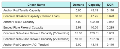
Hier sind die Ergebnisse Verhältnisse für alle ACI-Spannungsprüfungen:
Und hier sind die Ergebnisse Verhältnisse für alle ACI-Schernachweise:
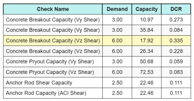
Wir erhalten den Scheck mit dem größten Verhältnis und vergleichen ihn mit dem maximalen Interaktionsverhältnis ACI 318-19 Gl. 17.8.3.
\(ICH_{int} = frac{N_{Tun}}{\phi N_n} + \frac{V_{Tun}}{\phi V_n} = frac{30}{47.749} + \frac{6}{17.921} = 0.96308\)
Schon seit 0.96 < 1.2, Die Interaktionsprüfung ist ausreichend.
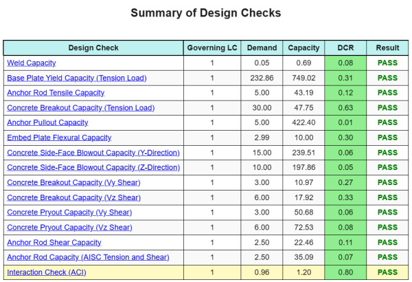
Entwurfszusammenfassung
Mit der Skyciv Base Plate Design Software kann automatisch einen Schritt-für-Schritt-Berechnungsbericht für dieses Entwurfsbeispiel erstellen. Es enthält auch eine Zusammenfassung der durchgeführten Schecks und deren resultierenden Verhältnisse, Die Informationen auf einen Blick leicht zu verstehen machen. Im Folgenden finden Sie eine Stichprobenzusammenfassungstabelle, Welches ist im Bericht enthalten.
SKYCIV -Beispielbericht
Sehen Sie sich den Detaillierungsgrad und die Klarheit an, die Sie von einem SkyCiv-Grundplatten-Designbericht erwarten können. Der Bericht umfasst alle wichtigen Designprüfungen, Gleichungen, und Ergebnisse werden in einem klaren und leicht lesbaren Format präsentiert. Es entspricht vollständig den Designstandards. Klicken Sie unten, um einen Beispielbericht anzuzeigen, der mit dem SkyCiv-Grundplattenrechner erstellt wurde.
Basisplattensoftware kaufen
Kaufen Sie die Vollversion des Basisplatten -Designmoduls selbst ohne andere Skyciv -Module selbst. Auf diese Weise erhalten Sie einen vollständigen Satz von Ergebnissen für die Basisplattendesign, Einbeziehung detaillierter Berichte und mehr Funktionen.