
In Stahlverbindungsausführung, Schrauben sind in der Regel als Schraubengruppe konzipiert, die als ein Körper fungiert und einer bestimmten Last standhält. Die Stärke einer Schraubengruppe wird normalerweise durch die steuernde Stärke ihrer kritischsten Schraube bestimmt. Die direkten Lasten werden auf die Gesamtzahl der Schrauben verteilt, während das induzierte Moment aufgrund der Lastexzentrizität im Verhältnis zum Trägheitsmoment der Schraubengruppe und zum Abstand vom Schwerpunkt verteilt wird. Dies wird als elastische Analyse bezeichnet. Aufgrund seiner vereinfachten und konservativen Annahmen zur Lastverteilung, es führt oft zu überdimensionierten Schraubverbindungen.
Wenn es um Value Engineering und wirtschaftliche Designs geht, Der unelastische Ansatz wird von den meisten Herstellern bevorzugt. Bei gleicher Belastung sind weniger Schrauben erforderlich. Um den unelastischen Ansatz zu machen, das momentane Rotationszentrum (ICOR) Methode mit Iterationen ist der beste Weg.
In diesem Artikel, Wir zeigen, wie man die Stärke von a berechnet Schraubverbindung mit der ICOR-Methode. Die Reaktionen pro Bolzen werden mithilfe der Gleichung berechnet (7-1) Auf Seite 7-7 des AISC-Handbuchs, 15. Ausgabe. Damit wird dann überprüft, ob die angenommene Lage des momentanen Mittelpunkts der Schraubengruppe korrekt ist. Schließlich, sobald wir den richtigen IC-Standort haben, Wir berechnen den Schraubengruppenkoeffizienten C, um seine Festigkeit zu bestimmen.
Von Hand gearbeitet, Die ICOR-Methode ist ein langer Prozess, weil das Momentane Zentrum gefunden wurde (IC) ist Versuch und Irrtum. Mit einem Computerlöser wird der IC einer Schraubengruppe stattdessen durch programmierte Iterationen ermittelt. Mit der SkyCiv Bolt Group Solver Verwendet eine schnelle Iterationsmethode, um die IC-Position und den Schraubengruppenkoeffizienten in Sekunden zu bestimmen. Es wird sowohl vom AISC als auch vom AS verwendet 4100 Anschlussmodule.
Das folgende Beispiel ist die gleiche Berechnung, die der Solver durchführt, Es wird eine lange Hand angezeigt, damit Sie verfolgen können, was es tut.
Abrufen der Schraubengruppeneigenschaften
Beginnen wir mit einer einfachen Analyse einer Schraubengruppe aus vier Schrauben, die mit einer exzentrischen vertikalen Scherlast von belastet sind 10 Kips. Die Exzentrizität der Last entlang der x-Achse beträgt 4 Zoll rechts von der Schraubengruppe. Der Winkel zur Vertikalen ist Null und die Exzentrizität entlang der y-Achse ist Null.
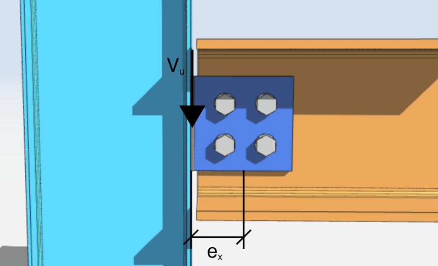
[math] V_{u} = 10\,kips [math]
[math] \theta = 0\,deg [math]
[math] e_{x} = 4\,in [math]
[math] e_{y} = 0\,in [math]
Als Erstes müssen die Koordinaten aller Schrauben in der Gruppe ermittelt werden. Visuelle Anleitungen und Tabellen werden dringend empfohlen.
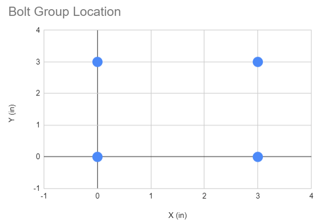
| Shop-ID | X. (im) | UND (im) |
| 1 | 0 | 0 |
| 2 | 0 | 3 |
| 3 | 3 | 0 |
| 4 | 3 | 3 |
Um den Schwerpunkt der Schraubengruppe entlang der x- und y-Achse zu ermitteln, Wir brauchen die folgende Formel.
Lassen [mathin] n [mathin] = Gesamtzahl der Schrauben
[math] X_{CG} = \frac{\sum X}{n} [math]
[math] Y_{CG} = \frac{\sum Y}{n} [math]
Dann, Unsere Lösung ist:
[math] X_{CG} = \frac{\sum X}{n} = \frac{0\,in + 0\,in + 3\,in + 3\,in}{4} = 1.5\,in [math]
[math] Y_{CG} = \frac{\sum Y}{n} = \frac{0\,in + 3\,in + 0\,in + 3\,in}{4} = 1.5\,in [math]
Angenommen, der Standort des I.C.
Nachdem Sie den Schwerpunkt erhalten haben, Wir nehmen die Lage des momentanen Zentrums an (IC). Als erster Versuch, Wir können davon ausgehen, dass der IC im geometrischen Schwerpunkt der Schraubengruppe sitzt.
So, davon ausgehen
[math] X_{IC} = X_{CG} = 1.5\,in [math]
[math] Y_{IC} = Y_{CG} = 1.5\,in [math]
Dann tabellieren wir die Verschiebung jedes Bolzens vom IC. Ermitteln Sie zunächst den Abstand entlang x und den Abstand entlang y, dann die resultierende Verschiebung.
| Shop-ID | cx (im) | cy (im) | c (im) |
| 1 | -1.5 | -1.5 | 2.121 |
| 2 | -1.5 | 1.5 | 2.121 |
| 3 | 1.5 | -1.5 | 2.121 |
| 4 | 1.5 | 1.5 | 2.121 |
Wo,
[math] c_{x} = X_{i} – X_{IC} [math]
[math] c_{y} = Y_{i} – Y_{IC} [math]
[math] c = \sqrt{ {\left( c_{x} \right)}^{2} + {\left( c_{y} \right)}^{2} } [math]
Für Schraube Nr. 1, Unsere Lösung ist
[math] c_{x} = 0\,in – 1.5\,in = -1.5\,in [math]
[math] c_{y} = 0\,in – 1.5\,in = -1.5\,in [math]
[math] c = \sqrt{ {\left( -1.5\,in \right)}^{2} + {\left( -1.5\,in \right)}^{2} } = 2.121\,in [math]
Berechnen Sie die Verformung pro Schraube bzgl. Abstand von IC
Nachdem Sie die Schraubenabstände vom angenommenen IC-Standort ermittelt haben, Wir berechnen die Verformung jedes Bolzens als Funktion seines Abstands.
Die maximale Verformung pro Schraube, [mathin] \Delta_{max} = 0.34\,in [mathin], basiert auf experimentellen Daten für eine ASTM-Schraube, wie auf der AISC-Seite beschrieben 7-8. Im linearen Verhältnis, und Einstellung [mathin] \Delta_{max} = 0.34\,in [mathin], Wir können die Verformung einer einzelnen Schraube im Verhältnis zu ihrem Anteil am maximalen Abstand berechnen [mathin] c_{max} [mathin]. Die Gleichung für das Erhalten [mathin] \Delta [mathin] wird unten gezeigt.
[math] \Delta_{1} = 0.34\,in \times \left( \frac{c}{c_{max}} \right) [math]
Für Schraube Nr. 1, die Verformung ist
[math] \Delta_{1} = 0.34\,in \times \left( \frac{2.121\,in}{2.121\,in} \right) = 0.34\,in [math]
Weil der IC im Schwerpunkt angenommen wurde, alle vier Schrauben haben den gleichen Abstand davon, alle vier erreichen also die gleiche Verformung. Die berechneten Verformungen sind unten tabellarisch aufgeführt.
| Shop-ID | [mathin] \Delta [mathin] (im) |
| 1 | 0.34 |
| 2 | 0.34 |
| 3 | 0.34 |
| 4 | 0.34 |
Holen Sie sich die Reaktionen pro Bolzen
Sobald wir die Verformung pro Schraube haben, Wir verwenden AISC 15. Ed. Gl (7-1) um die Reaktionen pro Schraube zu erhalten.
[math] R = R_{ult} \left( 1 – e^{-10\Delta} \right)^{0.55} [math]
Mit der [mathin] R_{ult} [mathin] in der Gleichung ist die angenommene Bruchlast einer Schraube, die wir als Schraubenscherfestigkeit einstellen können.
[math] R_{ult} = \phi R_{n} [math]
Für unser Beispiel, Wir verwenden eine Schraubenscherfestigkeit von [mathin] 24.4\,kip [mathin]. Ein anderer Wert ist gleichermaßen gültig, weil es sich aufhebt, wenn wir den Schraubengruppenkoeffizienten berechnen [mathin] C [mathin] später.
Für Schraube Nr. 1, die berechnete Reaktion ist
[math] R = R_{ult} \left( 1 – e^{-10\Delta} \right)^{0.55} [math]
[math] R = 24.4\,kip \left( 1 – e^{-10 \times \left( 0.34\,in \right)} \right)^{0.55} [math]
[math] R = 23.949\,kip [math]
Für den Rest der Schrauben, die berechneten Reaktionen sind wie folgt. Die Komponenten der Bolzenreaktion [mathin] R [mathin] entlang x und y sind ebenfalls gezeigt.
| Shop-ID | R. (kip) | Rx (kip) | Ry (kip) |
| 1 | 23.949 | 16.937 | -16.937 |
| 2 | 23.949 | -16.937 | -16.937 |
| 3 | 23.949 | 16.937 | 16.937 |
| 4 | 23.949 | -16.937 | 16.937 |
| ⅀Rx = 0 | ⅀Ry = 0 |
Jede Bolzenkraft wirkt senkrecht zu der Linie, die diesen Bolzen mit dem IC verbindet, Das ist es, was das Vorzeichen seiner beiden Komponenten festlegt. Für Schraube Nr. 1, Die Lösungen für die x- und y-Komponenten sind unten aufgeführt.
[math] R_{x} = -R \left( \frac{c_{y}}{c} \right) = -23.949 \times \left( \frac{-1.5\,in}{2.121\,in} \right) = 16.937\,kip [math]
[math] R_{y} = R \left( \frac{c_{x}}{c} \right) = 23.949 \times \left( \frac{-1.5\,in}{2.121\,in} \right) = -16.937\,kip [math]
Als nächstes benötigen wir den Moment, den jede Bolzenreaktion um den IC erzeugt. Verwenden Sie die Komponenten [mathin] R_{x} [mathin] und [mathin] R_{y} [mathin] mit den Hebelarmen [mathin] c_{y} [mathin] und [mathin] c_{x} [mathin].
[math] M_{r} = -R_{x} c_{y} + R_{y} c_{x} [math]
Für Schraube Nr. 1, Momentan ist die Reaktion auf den IC
[math] M_{r} = -16.937\,kip \times \left( -1.5\,in \right) + \left( -16.937\,kip \right) \times \left( -1.5\,in \right) [math]
[math] M_{r} = 50.811\,kip\text{-}in [math]
Als Scheck, der gleiche Moment ist [mathin] R \times c = 23.949 \times 2.121 = 50.8\,kip\text{-}in [mathin], weil die Kraft senkrecht zum Radius ist.
Jeder Bolzen sitzt hier im gleichen Abstand vom angenommenen IC und trägt die gleiche Kraft, Daher kehrt jeder Bolzen im selben Moment zurück. Die Momentreaktionen sind unten tabellarisch aufgeführt.
| Shop-ID | Herr (Hühnchen) |
| 1 | 50.811 |
| 2 | 50.811 |
| 3 | 50.811 |
| 4 | 50.811 |
| ⅀Herr = 203.244 |
Überprüfung des IC-Standorts
Jetzt haben wir die Scher- und Momentreaktionen pro Schraube, Wir verwenden sie, um die Belastung zu bestimmen, der diese Schraubengruppe standhält. Nehmen Sie die Resultierende aus der Summe aller Reaktionen entlang x und der Summe aller Reaktionen entlang y.
Aus dem vorherigen Abschnitt, Das haben wir berechnet
[math] \sum R_{x} = 0\,kip [math]
und
[math] \sum R_{y} = 0\,kip [math]
So,
[math] P_{u} = \sqrt{ {\left( \sum R_{x} \right)}^{2} + {\left( \sum R_{y} \right)}^{2} } = 0\,kip [math]
Die resultierende Belastung beträgt [mathin] P_{u} = 0\,kip [mathin]. Eine Schraubengruppe, die sich um ihren eigenen Schwerpunkt dreht, trägt ein reines Moment und keine Nettokraft, Daher kann es der ausgeübten Scherung nicht standhalten. Das zeigt uns bereits, dass der erste angenommene IC-Standort falsch ist, und wir könnten hier aufhören. Für den Zweck dieser Diskussion, Wir werden mit den restlichen Schritten fortfahren.
[math] P_{ux} = -P_{u}\sin\left( \theta \right) = 0\,kip [math]
[math] P_{uy} = -P_{u}\cos\left( \theta \right) = 0\,kip [math]
[math] M_{u} = -P_{ux}\left( Y_{CG} + e_{y} – Y_{IC} \right) + P_{uy} \left( X_{CG} + e_{x} – X_{IC} \right) = 0\,kip\text{-}in [math]
Schon seit,
[math] P_{ux} \neq \sum R_{x} [math]
[math] P_{uy} \neq \sum R_{y} [math]
[math] M_{u} \neq \sum M_{r} [math]
Das aufgebrachte Moment ist Null, während sich die Bolzenreaktionen summieren 203.244 Hühnchen, Das Gleichgewicht ist also nicht erfüllt. Der vermutete Standort des I.C. ist falsch, und wir bewegen uns zum nächsten angenommenen Ort.
SkyCiv hat die Schraubengruppenberechnung in seine Verbindungsdesignmodule integriert. Möchten Sie unsere Verbindungsdesign-Software ausprobieren?
Zweite Iteration
Für unsere zweite Iteration, Nehmen wir an, der I.C. befindet sich an den unten angegebenen Koordinaten. Denn die Last ist eine nach unten gerichtete Scherung, die rechts von der Gruppe ausgeübt wird, Der wahre IC liegt links vom Schwerpunkt, Der Prozess geht also in diese Richtung.
Davon ausgehen
[math] X_{IC} = 0.062\,in [math]
[math] Y_{IC} = 1.5\,in [math]
Wiederholen Sie dann die Schritte aus der ersten Iteration. Die folgende Tabelle zeigt die Koordinaten, der Abstand jedes Bolzens vom angenommenen I.C., und die entsprechende Verformung in Bezug auf diesen Abstand.
| Shop-ID | X. (im) | UND (im) | cx (im) | cy (im) | c (im) | [mathin] \Delta [mathin] (im) |
| 1 | 0 | 0 | -0.062 | -1.5 | 1.501 | 0.155 |
| 2 | 0 | 3 | -0.062 | 1.5 | 1.501 | 0.155 |
| 3 | 3 | 0 | 2.938 | -1.5 | 3.299 | 0.34 |
| 4 | 3 | 3 | 2.938 | 1.5 | 3.299 | 0.34 |
Diesmal haben die Bolzen nicht alle den gleichen Abstand vom IC, also erreicht nur das ferne Paar das 0.34 im Limit. Das nahe Paar verformt sich weniger und trägt daher weniger Last.
Beachten Sie, dass der berechnete Schwerpunkt des Schraubengruppe ist unverändert, da sich die Schraubenkoordinaten nicht verschoben haben.
[math] X_{CG} = 1.5\,in [math]
[math] Y_{CG} = 1.5\,in [math]
Dann berechnen wir die Reaktionen entlang x, die Reaktionen entlang y, und dem entsprechenden Moment. Die Werte sind unten tabelliert.
| Shop-ID | R. (kip) | Rx (kip) | Ry (kip) | Herr (Hühnchen) |
| 1 | 21.4 | 21.4 | -0.9 | 32.1 |
| 2 | 21.4 | -21.4 | -0.9 | 32.1 |
| 3 | 23.9 | 10.9 | 21.3 | 79.0 |
| 4 | 23.9 | -10.9 | 21.3 | 79.0 |
| ⅀Rx = 0 | ⅀Ry = 41 | ⅀Herr = 222 |
Als nächstes, wir bestimmen die resultierende Belastung aller Reaktionen entlang x und y.
[math] P_{u} = \sqrt{ {\left( \sum R_{x} \right)}^{2} + {\left( \sum R_{y} \right)}^{2} } [math]
[math] P_{u} = \sqrt{ {\left( 0\,kip \right)}^{2} + {\left( 40.703\,kip \right)}^{2} } [math]
[math] P_{u} = 40.703\,kip [math]
Dann die Komponenten der resultierenden Last, basierend auf dem Gegebenen [mathin] \theta [mathin], sind unten dargestellt.
[math] P_{ux} = -P_{u}\sin\left( \theta \right) = -41\,kip \times \sin\left( 0\,deg \right) = 0\,kip [math]
[math] P_{uy} = -P_{u}\cos\left( \theta \right) = -41\,kip \times \cos\left( 0\,deg \right) = -41\,kip [math]
Anschließend verwenden wir diese Komponenten, um die Momentenlast über den angenommenen I.C. zu ermitteln.
[math] M_{u} = -P_{ux} \left( Y_{CG} + e_{y} – Y_{IC} \right) + P_{uy} \left( X_{CG} + e_{x} – X_{IC} \right) [math]
[math] M_{u} = -0\,kip \left( 1.5\,in + 0\,in – 1.5\,in \right) + \left( -41\,kip \right) \left( 1.5\,in + 4\,in – 0.062\,in \right) [math]
[math] M_{u} = -222\,kip\text{-}in [math]
Als nächstes, vergleichen wir die errechneten [mathin] P_{ux} [mathin], [mathin] P_{uy} [mathin] und [mathin] M_{u} [mathin] gegen die Reaktionen der Bolzengruppe.
[math] P_{ux} \approx -\sum R_{x} [math]
[math] P_{uy} \approx -\sum R_{y} [math]
[math] M_{u} \approx -\sum M_{r} [math]
Das ist numerisch 0 gegen 0, -41 gegen kippen -41 kip, und -222 Kip-in gegen -222 Hühnchen. Die linke Seite liegt nahe genug an der rechten Seite, sodass wir den vermuteten Standort des I.C. erkennen können. als richtig.
In der Praxis verschiebt der Solver den Versuchs-IC so lange, bis diese drei Residuen innerhalb einer Toleranz liegen, anstatt bei einer visuellen Übereinstimmung stehenzubleiben.
Auflösen nach dem C-Koeffizienten
Sobald der I.C. Standort bestimmt, Mit der folgenden Formel können wir den Schraubengruppenkoeffizienten C ermitteln.
[math] C = \frac{P_{u}}{\phi R_{n}} = \frac{40.703\,kip}{24.4\,kip} = 1.668 [math]
Der Koeffizient bedeutet, dass die Gruppe trägt 1.668 mal so stark wie eine einzelne Schraube. Beachten Sie, dass dies deutlich unter den vier vorhandenen Schrauben liegt, weil die Exzentrizität die Gruppe den größten Teil ihrer Nennkapazität kostet. Hier liegt auch die Wahl [mathin] R_{ult} [mathin] storniert, Aus diesem Grund könnte am Anfang jeder konsistente Wert verwendet werden.
Kostenloser Schraubengruppenrechner
Sehen Sie im Verbindungsdesign-Modul, wie wir unsere Schraubverbindungen mit diesem Ansatz entwerfen. Wählen Sie eine Schraubverbindung, Stellen Sie die Schraubenanordnung und die Exzentrizität ein, und der Bericht gibt die IC-Position und den C-Koeffizienten zusammen mit jeder anderen Überprüfung an. Es läuft im Browser, ohne dass es etwas zu installieren gibt.
Für mehr Funktionalität, einschließlich Speichern und erneutes Laden Ihrer Dateien, Melden Sie sich für ein kostenloses Konto an.
