So berechnen Sie die maximale Tragfähigkeit eines einzelnen Pfahls

Tragfähigkeit

---

Die Bewertung der endgültigen Tragfähigkeit eines einzelnen Pfahls ist einer der wichtigsten Aspekte der Pfahlkonstruktion, und kann manchmal kompliziert sein. In diesem Artikel werden die maßgeblichen Gleichungen für die Einzelpfahlkonstruktion sowie ein Beispiel erläutert.

Den Lastübertragungsmechanismus eines einzelnen Pfahls leicht verstehen, Stellen Sie sich einen Betonpfahl der Länge L und des Durchmessers D vor, wie in Abbildung gezeigt 1.

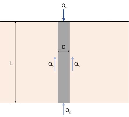
Abbildung 1: Lastübertragungsmechanismus für Pfähle

Die auf den Pfahl wirkende Last Q muss direkt auf den Boden am Pfahlboden übertragen werden. Ein Teil dieser Last wird von den Seiten des Pfahls aufgenommen, und zwar mithilfe von etwas, das sog “Hautreibung” entlang des Schaftes entwickelt (Q._s), und dem Rest wird der Boden widerstehen, auf dem der Pfahl ruht (Q._p). Deshalb, die ultimative Tragfähigkeit (Qu) eines Pfahls ergibt sich aus der Gleichung (1). Es stehen mehrere Methoden zur Schätzung der Werte von Q zur Verfügung_p und Q_s.

\( {Q.}_{u} = {Q.}_{p} + {Q.}_{s} \) (1)

Q._u = maximale Tragfähigkeit

Q._p = Endlagertragfähigkeit

Q._s = Hautreibungswiderstand

Möchten Sie die Foundation Design-Software von SkyCiv ausprobieren?? Unser kostenloses Tool ermöglicht es Benutzern, Tragfähigkeitsberechnungen durchzuführen, ohne dass ein Download oder eine Installation erforderlich ist!

Foundation Design Calculator

Endtragfähigkeit, Q._p

---

Die ultimative Endtragfähigkeit ist theoretisch die maximale Belastung pro Flächeneinheit, die der tragende Boden tragen kann, ohne Scheitern. Die folgende Gleichung von Karl Von Terzaghi, der Vater der Bodenmechanik, ist eine der ersten und am häufigsten verwendeten Theorien zur Bewertung der endgültigen Tragfähigkeit von Fundamenten. Die Terzaghi-Gleichung für die ultimative Tragfähigkeit kann wie folgt ausgedrückt werden::

\( {q}_{u} = (c × {N.}_{c}) + (q × {N.}_{q}) + (\frac{1}{2} × c × B × {N.}_{γ }) \) (2)

q_u = Ultimative Endtragfähigkeit

c = Kohäsion des Bodens

q = Effektiver Bodendruck

γ = Bodeneinheitsgewicht

B = Querschnittstiefe oder -durchmesser

N._c, N._q, N._γ = Lagerfaktoren

Da q_u bezieht sich auf die Belastung pro Flächeneinheit oder Druck, Durch Multiplizieren mit der Querschnittsfläche des Pfahls erhält man die Endtragfähigkeit (Q._p) des Stapels. Der resultierende Wert des letzten Termes der Gleichung 2 ist aufgrund einer relativ geringen Florbreite vernachlässigbar, daher, es kann aus der Gleichung gestrichen werden. So, Die maximale Endtragfähigkeit des Pfahls kann wie in der Gleichung dargestellt ausgedrückt werden (3). Diese modifizierte Version der Terzaghi-Gleichung wird im SkyCiv Foundation-Modul beim Entwerfen von Pfählen verwendet.

\( {Q.}_{p} = {Ein}_{p} × [(c × {N.}_{c}) + (q × {N.}_{q}) ] \) (3)

Ein_p = Querschnittsfläche des Pfahls

Lagerfaktoren N_c und N_q sind nichtdimensional, empirisch abgeleitet, und sind Funktionen des Bodenreibungswinkels (Phi). Die zur Ermittlung der Lagerfaktoren erforderlichen Berechnungen haben die Forscher bereits abgeschlossen. Tabelle 1 fasst die Werte von N zusammen_q nach Angaben des Naval Facilities Engineering Command (NAVFAC DM 7.2, 1984). Der Wert von N_c ist ungefähr gleich 9 für Pfähle unter lehmigen Böden.

Lagerfaktor (N.q)
Reibungswinkel (Ö)	26	28	30	31	32	33	34	35	36	37	38	39	40
Rammpfähle	10	15	21	24	29	35	42	50	62	77	86	120	145
Gelangweilte Haufen	5	8	10	12	14	17	21	25	30	38	43	60	72

Tabelle 1: N._q Werte aus NAVFAC DM 7.2

Hautreibungswiderstandskapazität, Q._s

---

Der Hautreibungswiderstand von Pfählen entwickelt sich entlang der Pfahllänge. Allgemein, Der Reibungswiderstand eines Pfahls wird ausgedrückt als:

\( {Q.}_{s} = ∑ (p × ΔL × f) \) (4)

p = Umfang des Pfahls

ΔL = Inkrementelle Pfahllänge, über die p und f gemessen werden

f = Reibungswiderstandseinheit in jeder Tiefe

Schätzung des Wertes des Reibungswiderstands der Einheit (f) erfordert die Berücksichtigung mehrerer wichtiger Faktoren, wie die Art der Pfahlinstallation und die Bodenklassifizierung. Gleichungen (5) und (6) zeigt die Berechnungsmethode zur Ermittlung des Einheitsreibungswiderstands von Pfählen in sandigen und tonigen Böden, beziehungsweise. Tabellen 2 und 3 Geben Sie den empfohlenen effektiven Erddruckbeiwert an (K.) und der Boden-Haufen-Reibungswinkel (D'), gemäß NAVFAC DM7.2.

Für sandige Böden:

\( Für f = K × σ’×(D') \) (5)

K = Effektiver Erddruckbeiwert

σ’ = Effektive Vertikalspannung in der betrachteten Tiefe

D’ = Reibungswinkel Boden-Haufen

Für lehmige Böden:

\( f = a × c \) (6)

α = Empirischer Adhäsionsfaktor

Reibungswinkel Boden-Pfahl (D')
Pfahltyp	D’
Stahlpfahl	20Um es zu berechnen
Holzstapel	3/4 × F
Betonpfahl	3/4 × F

Tabelle 2: Werte des Boden-Pfahl-Reibungswinkels (NAVFAC DM7.2, 1984)

Lateraler Erddruckkoeffizient (K.)
Pfahltyp	Kompressionspfahl	Spannungspfahl
Gerammte H-Pfähle	0.5-1.0	0.3-0.5
Rammverdrängungspfähle (runden, rechteckig)	1.0-1.5	0.6-1.0
Rammverdrängungspfähle (konisch)	1.5-2.0	1.0-1.3
Rammpfähle	0.4-0.9	0.3-0.6
Gelangweilte Pfähle (<24″ Durchmesser)	0.7	0.4

Tabelle 3: Lateraler Erddruckkoeffizient (K.) Werte (NAVFAC DM7.2, 1984)

Adhäsionsfaktor (ein)
c/pein	ein
≤ 0.1	1.00
0.2	0.92
0.3	0.82
0.4	0.74
0.6	0.62
0.8	0.54
1.0	0.48
1.2	0.42
1.4	0.40
1.6	0.38
1.8	0.36
2.0	0.35
2.4	0.34
2.8	0.34

Hinweis: p_ein = Atmosphärendruck ≈ 100 kN / m²

Tabelle 4: Werte des Adhäsionsfaktors (p-Delta-Effekte, Picken, und Mesri, 1996)

Beispiel: Berechnung der Tragfähigkeit von Pfählen im Sand

---

Ein 12 Meter langer Betonpfahl mit einem Durchmesser von 500 mm wird in mehrere Sandschichten gerammt, ohne dass Grundwasser vorhanden ist. Finden Sie die ultimative Tragfähigkeit (Q._u) des Stapels.

Einzelheiten
Sektion
Durchmesser	500 mm
Länge	12 Mio.
Layer 1-Bodeneigenschaften
Dicke	5 Mio.
Gewichtseinheit	17.3 kN / m3
Reibungswinkel	30 Abschlüsse
Zusammenhalt	0 kPa
Grundwasserspiegel	Nicht anwesend
Layer 2-Bodeneigenschaften
Dicke	7 Mio.
Gewichtseinheit	16.9 kN / m3
Reibungswinkel	32 Abschlüsse
Zusammenhalt	0 kPa
Grundwasserspiegel	Nicht anwesend

Schritt 1: Berechnen Sie die Tragfähigkeit des Endlagers (Q._p).

An der Spitze des Stapels:

Ein_p = (S./4) Axiale Tragfähigkeit des Pfahls² = (S./4) × 0.5²

Ein_p = 0.196 Mio.²

c = 0 kPa

θ = 32º

N._q = 29 (Aus der Tabelle 1)

Effektiver Bodendruck (q):

q = (γ ₁ × t₁) + (γ ₂ × t₂) = (5 m × 17.3 kN / m³) + (7 m × 16.9 kN / m³)

q = 204.8 kPa

Dann verwenden Sie die Gleichung (3) für die Endtragfähigkeit:

Q._p = Ein_p × [(c × N_c) + (q × N_q)]

Q._p = 0.196 Mio.² × ( 204.8 KPa × 29)

Q._p = 1,164.083 kN

Schritt 2: Berechnen Sie den Hautreibungswiderstand (Q._s).

Gleichungen verwenden (4) und (5), Berechnen Sie die Hautreibung pro Bodenschicht.

Q._s = ∑ (p × ΔL × f)

p = π × D = π × 0.5 Mio.

p = 1.571 Mio.

Ebene 1:

L = 5 Mio.

f₁ = K × p’₁× braun(D')

K = 1.25 (Tabelle 3)

D’ = 3/4 × 30º

D’ = 22,50º

σ’₁ = c₁ × (0.5 × t₁) = 17.3 kN / m³ × (0.5 × 5 Mio.)

σ’₁ = 43.25 kN / m²

f₁ = 1.25 × 43.25 kN / m² × braun(22.50Um es zu berechnen)

f₁ = 22.393 kN / m²

Q._s1 = p × ΔL × f₁ = 1.571 m × 5 m × 22.393 kN / m²

Q._s1 = 175.897 kN

Ebene 2:

L = 7 Mio.

f₂ = K × p’₂× braun(D')

K = 1.25 (Tabelle 3)

D’ = 3/4× 32º

D’ = 24º

σ’₂ = (γ ₁ × t₁) + [γ ₂ × (0.5 × t₂)] = (17.3 kN / m³ × 5 Mio.) + [16.9 kN / m³ ×(0.5 × 7 Mio.)]

σ’₂ = 145.65 kN / m²

f₂ = 1.25 × 145.65 kN / m² × braun(24Um es zu berechnen)

f₂ = 81.059 kN / m²

Q._s2 = p × ΔL × f₂ = 1.571 m × 7 m × 81.059 kN / m²

Q._s2 = 891.406 kN

Vollständiger Reibungswiderstand der Haut:

Q._s = Q_s1+ Q._s2 = 175.897 kN + 891.406 kN

Q._s = 1,067.303 kN

Schritt 3: Berechnen Sie die maximale Tragfähigkeit (Q._u).

Q._u = Q_p+ Q._s = 1,164.083 kN + 1,067.303 kN

Q._u = 2,231.386 kN

Beispiel 2: Berechnung der Kapazität von Pfählen aus Ton

---

Betrachten Sie a 406 Betonpfahl mit mm Durchmesser und einer Länge von 30 m schichtweise eingebettet, gesättigter Ton. Finden Sie die ultimative Tragfähigkeit (Q._u) des Stapels.

Einzelheiten
Sektion
Durchmesser	406 mm
Länge	30 Mio.
Layer 1-Bodeneigenschaften
Dicke	10 Mio.
Gewichtseinheit	8 kN / m3
Reibungswinkel	0Um es zu berechnen
Zusammenhalt	30 kPa
Grundwasserspiegel	5 Mio.
Layer 2-Bodeneigenschaften
Dicke	10 Mio.
Gewichtseinheit	19.6 kN / m3
Reibungswinkel	0Um es zu berechnen
Zusammenhalt	0 kPa
Grundwasserspiegel	Vollständig untergetaucht

Schritt 1: Berechnen Sie die Tragfähigkeit des Endlagers (Q._p).

An der Spitze des Stapels:

Ein_p = (S./4) Axiale Tragfähigkeit des Pfahls²= (S./4) × 0.406²

Ein_p = 0.129 Mio.²

c = 100 kPa

N._c = 9 (Typischer Wert für Ton)

Q._p = (c × N_c) × A_p = (100 kPa × 9) × 0.129 Mio.²

Q._p = 116.1 kN

Schritt 2: Berechnen Sie den Hautreibungswiderstand (Q._s).

Gleichungen verwenden (4) und (6), Berechnen Sie die Hautreibung pro Bodenschicht.

Q._s = ∑ (p × ΔL × f)

p = π × D = π × 0.406 Mio.

p = 1.275 Mio.

Ebene 1:

L = 10 Mio.

ein₁ = 0.82 (Tabelle 4)

c₁ = 30 kPa

f₁= a₁ × c₁ = 0.82 × 30 kPa

f₁ = 24.6 kN / m²

Q._s1 = p × ΔL × f₁ = 1.275 m × 10 m × 24.6 kN / m²

Q._s1 = 313.65 kN

Ebene 2:

L = 20 Mio.

ein₂= 0.48 (Tabelle 4)

c₂ = 100 kPa

f₂ = a₂ × c₂ = 0.48 × 100 kPa

f₂ = 48 kN / m²

Q._s2 = p × ΔL × f₂ = 1.275 m × 20 m × 48 kN / m²

Q._s2 = 1,224 kN

Vollständiger Reibungswiderstand der Haut:

Q._s = Q_s1+ Q._s2 = 313.65 kN + 1224 kN

Q._s = 1,537.65 kN

Schritt 3: Berechnen Sie die maximale Tragfähigkeit (Q._u).

Q._u = Q_p+ Q._s = 116.1 kN + 1537.65 kN

Q._u = 1,653.75 kN

Möchten Sie die Foundation Design-Software von SkyCiv ausprobieren?? Unser kostenloses Tool ermöglicht es Benutzern, Tragfähigkeitsberechnungen durchzuführen, ohne dass ein Download oder eine Installation erforderlich ist!

Foundation Design Calculator

Verweise:

• Das, B.M. (2007). Grundlagen des Grundbaus (7th Ausgabe). Globales Engineering
• Rajapakse, R.. (2016). Faustregel für Pfahldesign und -konstruktion (2nd Ausgabe). Elsevier Inc.
• Tomlinson, M.J. (2004). Pfahlentwurfs- und Baupraxis (4th Ausgabe). E. & Sponser der Vereinten Nationen.