Von der Norm berücksichtigte Plattensysteme
Australische Normen legen die Mindestanforderungen für die Bemessung von Stahlbetonplatten fest, wie Einweg- und Zweiwegtypen. Hinsichtlich der Plankonfiguration und der Aufnahme von Balken, Die Platten können auch in vierseitig gelagerte Platten unterteilt werden, Träger-Platten-Systeme, flache Platten, und Flachplatten. Diese Typen sind in den folgenden Bildern zusammengefasst.
Vereinfachen Sie die Einhaltung der australischen Plattenkonstruktion mit den erweiterten Funktionen von SkyCiv Integrierter Beton Design-Module. Probieren Sie es aus! Tragen Sie AS ganz einfach auf 3600 prüft auf Brammen und flache Platten.
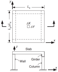
Abbildung 1. Platte auf vier Seiten gestützt. (Yew-Chaye Loo & Sanual Hug Chowdhury , “Bewehrter und vorgespannter Beton”, 22. Auflage, Cambridge University Press).
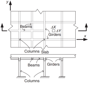
Abbildung 2. Grillplattensystem. (Yew-Chaye Loo & Sanual Hug Chowdhury , “Bewehrter und vorgespannter Beton”, 22. Auflage, Cambridge University Press).
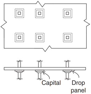
Abbildung 3. Flache Platten. (Yew-Chaye Loo & Sanual Hug Chowdhury , “Bewehrter und vorgespannter Beton”, 22. Auflage, Cambridge University Press).
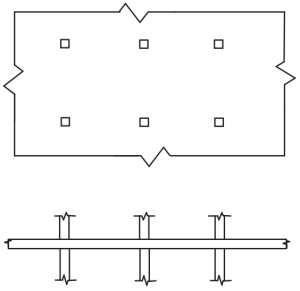
Abbildung 4. Flache Platten. (Yew-Chaye Loo & Sanual Hug Chowdhury , “Bewehrter und vorgespannter Beton”, 22. Auflage, Cambridge University Press).
Der Standard empfiehlt einige Methoden (vereinfachte und bewährte Verfahren) bei der Ermittlung von Biegemomenten:
- Klausel 6.10.2: Durchlaufträger und Einwegplatten
- Klausel 6.10.3: Vierseitig gelagerte Zwei-Wege-Platten
- Klausel 6.10.4: Zweiwegplatten mit mehreren Spannweiten
Der Zweck des Codes besteht darin, die Gesamtmenge an Bewehrungsstahl in Hauptrichtungen im Plattensystem zu bemessen. Bewehrungsstahl wird für die Biegemomente berechnet “Mx” und “Mein.” Abbildung 5 zeigt die anderen Kräfte oder Einwirkungen in einem endlichen Plattenelement, in dem der Code ihre Widerstandswerte vorschreibt.
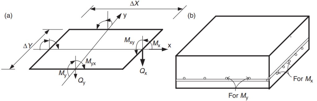
Abbildung 5. Kräfte in einem endlichen Plattenelement: Biegemomente (Mx, Meine), verdrehte Momente (Mxy, Myx), und Scheren (Qx, Qy). (Yew-Chaye Loo & Sanual Hug Chowdhury , “Bewehrter und vorgespannter Beton”, 22. Auflage, Cambridge University Press)
In diesem Artikel, Wir werden zwei Beispiele für Plattendesigns entwickeln, Einweg- und Zweiweg-Plattensysteme, unter Verwendung der vereinfachten Methoden, die sich am Code orientieren und erlauben. In beiden Fällen, Wir werden ein SkyCiv S3D-Modell erstellen und die Ergebnisse mit den oben genannten Methoden vergleichen.
Wenn Sie neu bei SkyCiv sind, Melden Sie sich an und testen Sie die Software selbst!
Beispiel für ein Einwegplattendesign
Unten sehen Sie das kleine Gebäude und die Platten, die wir entwerfen werden
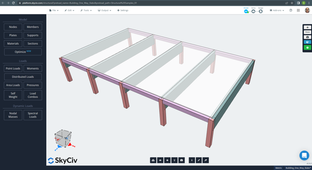
Abbildung 6. Einwegplatten in einem kleinen Gebäudebeispiel. (Strukturelles 3D, SkyCiv Cloud Engineering).
Die Planmaße werden nachfolgend angezeigt
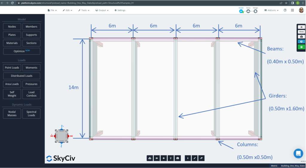
Abbildung 7. Planen Sie Abmessungen und Strukturelemente. (Strukturelles 3D, SkyCiv Cloud Engineering).
Für das Plattenbeispiel, Zusammenfassend, das Material, Elementeigenschaften, und jede Menge zu bedenken :
- Klassifizierung des Plattentyps: Eins – Art und Weise Verhalten \(\frac{L_2}{L_1} > 2 ; \frac{14 Mio.}{6 Mio.}=2,33 > 2.00 \) OK!
- Gebäudebesetzung: Wohnnutzung
- Plattendicke \(t_{Platte}=0.25m\)
- Stahlbetondichte unter der Annahme eines Stahlverstärkungsverhältnisses von 0.5% \(\rho_w = 24 \frac{kN}{m^3} + 0.6 \frac{kN}{m^3} \mal 0.5 = 24.3 \frac{kN}{m^3} \)
- Charakteristische Betondruckfestigkeit bei 28 Tage \(f’c = 25 MPa \)
- Konkreter Elastizitätsmodul nach australischem Standard \(E_c = 26700 MPa \)
- Eigengewicht der Platte \(Dead = \rho_w \times t_{Platte} = 24.3 \frac{kN}{m^3} \mal 0,25m = 6.075 \frac {kN}{m^2}\)
- Überlagerte Eigenlast \(SD = 3.0 \frac {kN}{m^2}\)
- Live-Last \(L = 2.0 \frac {kN}{m^2}\)
Handberechnung nach AS3600-Standard
In diesem Abschnitt, Wir berechnen den erforderlichen Bewehrungsstahl anhand der Referenz des australischen Standards. Wir ermitteln zunächst das gesamte faktorisierte Biegemoment, das auf den einheitlichen Breitenstreifen der Platte ausgeübt werden muss.
- Eigengewicht, \(g = (3.0 + 6.075) \frac{kN}{m^2} \mal 1 m = 9.075 \frac{kN}{ Mio.}\)
- Live-Last, \(q = (2.0) \frac{kN}{m^2} \mal 1 m = 2.0 \frac{kN}{ Mio.}\)
- Grenzlast, \(Fd = 1.2\times g + 1.5\mal q = (1.2\mal 9.075 + 1.5\mal 2.0)\frac{kN}{ Mio.} =13.89 \frac{kN}{ Mio.} \)
Verwendung der durch die Norm vorgegebenen vereinfachten Methode, zuerst, Es ist zwingend erforderlich, die folgenden Einschränkungen einzuhalten:
- \(\frac{L_i}{L_j} \das 1.2 . \frac{6 Mio.}{6 Mio.} =1 < 1.2 \). OK!
- Die Belastung muss gleichmäßig sein. OK!
- \(q \le 2g. q=2 \frac{kN}{ Mio.} < 18.15 \frac{kN}{ Mio.}\). OK!
- Der Plattenquerschnitt muss gleichmäßig sein. OK!.
Empfohlene Mindestdicke, d
\(d \ge \frac{L_{z.B}}{{k_3}{k_4}{\sqrt[3]{\frac{\frac{\p-Delta-Effekte}{L_{ef}}{E_c}}{F_{d, ef}}}}}\)
Wo
- \(k_3 = 1.0; k_4 = 1.75 \)
- \(\frac{\p-Delta-Effekte}{L_{ef}}=1/250 \)
- \(E_c = 27600 MPa \)
- \(F_{d,ef} = (1.0 +k_{cs})\mal g + (\psi_s + k_{cs}\times \psi_1) \mal q=(1.0+0.8)\mal 9.075 + (0.7+0.8\mal 0.4)\mal 2 = 18.375 kPa\)
- \(\psi_s = 0.7 \) Nutzlast-Kurzzeitfaktor
- \(\psi_1 = 0.4 \) Nutzlast-Langzeitfaktor
- \(k_{cs} = 0.8 \)
\(d \ge \frac{5.50 Mio.}{{1.0}\mal {1.75}{\sqrt[3]{\frac{\frac{1}{250}\mal{27600 \mal 10^3 kPa}}{18.375 kPa}}}} \ge 0,173m. d = 0,25m > 0.173 Mio. \) OK!
Sobald wir zeigen, dass die Einschränkungen erfüllt sind, Das Biegemoment wird mit dem Ausdruck berechnet: \(M=\alpha \times F_d \times L_n^2\) wo \(\Alpha) ist eine in der folgenden Abbildung definierte Konstante.
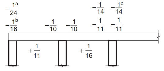
Abbildung 8. Werte des Momentkoeffizienten \(\Alpha) für Platten mit mehr als zwei Spannweiten. (Yew-Chaye Loo & Sanual Hug Chowdhury , “Bewehrter und vorgespannter Beton”, 22. Auflage, Cambridge University Press).
Wo:
- (ein) Fall von Platten und Trägern auf Trägerauflage
- (b) Nur für durchgehende Balkenunterstützung
- (c) Wo Bewehrung der Klasse L verwendet wird
- \(L_n \) ist die einheitliche Streifenspanne
- \(F_d \) ist die gravitationsfaktorisierte Last
Für das Plattenbeispiel, Wir müssen einen Anwendungsfall verwenden (ein) denn die Platte ruht auf steifen Trägern. Es wird nur ein Fall erläutert und der Rest wird in der folgenden Tabelle angezeigt. Wir berücksichtigen auch die Berechnung der Stahlverstärkungsfläche.
- \(M={\Alpha} {F_d}{L_n^2}={-\frac{1}{24}}\mal {13.89 \frac{kN}{ Mio.}}\mal (6 Mio.-0.5 Mio.)^2 = – 17.51{kN}{ Mio.}\)
- Abdeckung = 20 mm (Für die Feuerwiderstandsdauer sind mindestens 10 mm erforderlich 60 Minuten).
- \(d = t_{Platte} – Abdeckung – \frac{Stabdurchmesser}{2} = 250mm – 20mm – 6mm = 224 mm \)
- \(\alpha_2 = 1.0-0.003 f’c = 1.0-0.003\times 25 = 0.925 (0.67 \le \alpha_2 \le 0.85) \) So, wir wählen \(\alpha_2 = 0.85\)
- \(\xi = \frac{\alpha_2\times f’c}{f_{seine}} = frac{0.85\mal 25 MPa}{500 MPa} = 0.0425 \)
- \(\rho_t = \xi – \sqrt{{\xi}^ 2 – \frac{{2}{\xi}{M.}}{{\phi}{b}{d^2}{f_{seine}}}} = 0.0425 – \sqrt{{0.0425}^2-\frac{2\times 0.0425\times 17.51{kN}{ Mio.}}{{0.8}\mal {1 Mio.}\mal {{(0.224 Mio.)^ 2}} \mal {500\mal {10^ 3}kPa}}}=0.0008814\)
- \(\gamma= 1.05-0.007 f’c = 1.05-0.007\times 25 = 0.875 (0.67 \le \gamma \le 0.85) \) So, wir wählen \(\Gamma = 0.85\)
- \(k_u = \frac{\rho_t \times f_{seine}}{0.85\times \gamma \times f’c}= frac{0.0008814\mal 500 MPa}{0.85\mal 0.85 \mal 25 MPa} =0.0244\)
- \(\phi = 1.19 – \frac{13\mal k_{u0}}{12} = 1.19 – \frac{13\mal 0.0244}{12} = 1.164 (0.6 \le \phi \le 0.8) \) So, wir wählen \(\phi = 0.8\). OK!.
- \(\rho_{t,Min.} = 0.20 {(\frac{D.}{d})^ 2}{(\frac{f’_{ct,f}}{f_{seine}})} = 0.20 \mal (\frac{0.25 Mio.}{0.224 Mio.})^2 \times \frac{0.6\mal sqrt{25MPa}}{500 MPa} = 0.0015\)
- \(EIN_{st}=max(\rho_{t,Min.}, \rho_t)\times b \times d = max(0.0015,0.0008814)\mal 1000 mm \times 224 mm = 334.82 mm^2 \)
| \(\Alpha) und Momente | Äußere negative Linke | Äußerlich positiv | Äußeres negatives Recht | Innere negative Linke | Innen positiv | Inneres negatives Recht |
|---|---|---|---|---|---|---|
| \(\Alpha) Wert | -\(\frac{1}{24}\) | \(\frac{1}{11}\) | -\(\frac{1}{10}\) | \(\frac{1}{10}\) | \(\frac{1}{16}\) | \(\frac{1}{11}\) |
| M-Wert | -17.51 | 38.20 | -42.02 | 42.02 | 26.26 | 38.20 |
| \(\rho_t\) | 0.0008814 | 0.001948 | 0.002148 | 0.002148 | 0.00133 | 0.001948 |
| Zu | 0.0244 | 0.0539 | 0.0594 | 0.0594 | 0.0368 | 0.05391 |
| \(\Phi) | 0.8 | 0.8 | 0.8 | 0.8 | 0.8 | 0.8 |
| \(EIN_{st} {mm^2}\) | 334.82 | 436.31 | 481.099 | 481.099 | 334.8214 | 436.3100 |
Nach der Berechnung der Stahlbewehrungsfläche, Sie können die Detaillierung definieren (die tatsächliche Art und Weise, wie die Bewehrung in der Platte platziert wird). Als Hilfe für Ihr Wissen, Wir teilen das folgende Bild, Dies gibt die Position der Bewehrung für positive und negative Momente an:
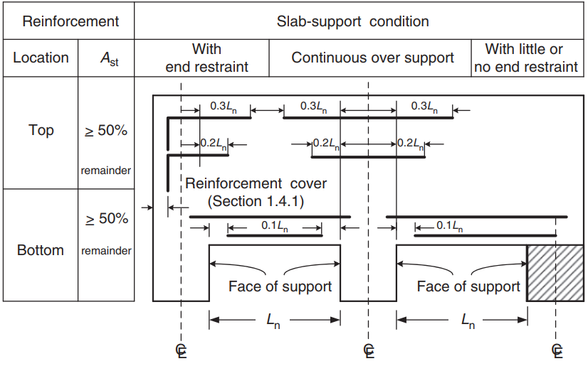
Abbildung 9. Bewehrungsanordnung für Einbahn- und Zweibahnplatten. (Yew-Chaye Loo & Sanual Hug Chowdhury , “Bewehrter und vorgespannter Beton”, 22. Auflage, Cambridge University Press)
Wenn Sie neu bei SkyCiv sind, Melden Sie sich an und testen Sie die Software selbst!
Ergebnisse des SkyCiv S3D Plate Design-Moduls
Auf den ersten Blick, Wir zeigen einige Bilder zur Modellierung und Strukturanalyse des Beispiels in S3D. Wir empfehlen Ihnen, über die folgenden Links mehr über die Modellierung in SkyCiv zu lesen So modellieren Sie Platten? Jedes Mal, wenn Sie eine neue hinzufügen Beispiel für ein ACI-Plattendesign mit SkyCiv.
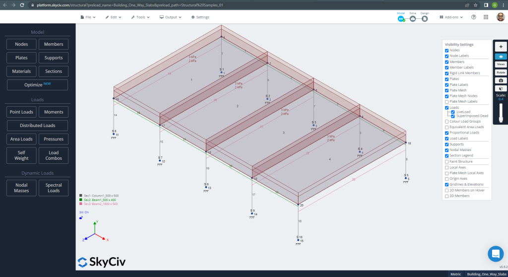
Abbildung 10. Strukturmodell in S3D für ein Beispiel für Einwegplatten. (Strukturelles 3D, SkyCiv Cloud Engineering).
Vor der Analyse des Modells, Wir müssen eine Plattenmaschenweite definieren. Einige Referenzen (2) Empfehlen Sie eine Größe für das Schalenelement von 1/6 der kurzen Spanne bzw 1/8 der langen Spanne, der kürzere von ihnen. Diesem Wert folgen, wir haben \(\frac{L2}{6}= frac{6 Mio.}{6} = 1 m \) oder \(\frac{L1}{8}= frac{14 Mio.}{8}=1,75m \); Als maximale empfohlene Größe gehen wir von 1 m und von der angewandten Maschenweite von 0,50 m aus.
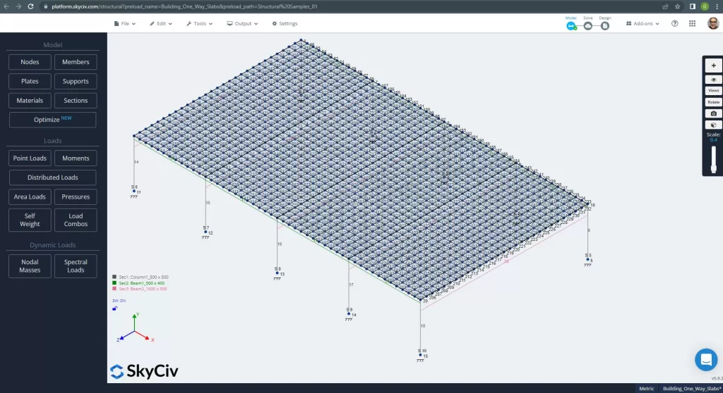
Abbildung 11. Verbessertes Netz in Platten. (Strukturelles 3D, SkyCiv Cloud Engineering).
Einmal haben wir unser analytisches Strukturmodell verbessert, Wir führen eine lineare elastische Analyse durch. Beim Entwerfen von Platten, Wir müssen prüfen, ob die vertikale Verschiebung kleiner als das vom Code zulässige Maximum ist. Australische Standards haben eine maximale vertikale Verschiebung der Wartungsfreundlichkeit festgelegt \(\frac{L.}{250}= frac{6000mm}{250}=24.0 mm\).
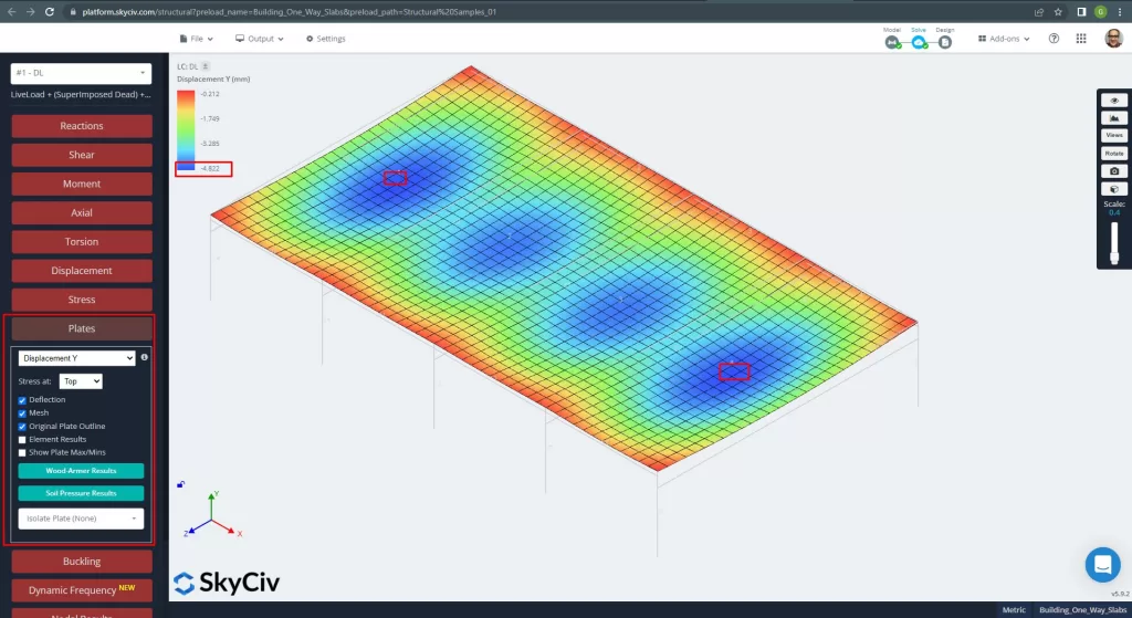
Abbildung 12. Vertikale Verschiebung in Platten. (Strukturelles 3D, SkyCiv Cloud Engineering).
Vergleich der maximalen vertikalen Verschiebung mit dem Code-Referenzwert, Die Steifigkeit der Platte ist ausreichend. \(4.822 mm < 24.00mm).
Die maximalen Momente in den Spannweiten der Platte liegen positiv in der Mitte und negativ an den Außen- und Innenstützen. Sehen wir uns diese Momentwerte in den folgenden Bildern an.
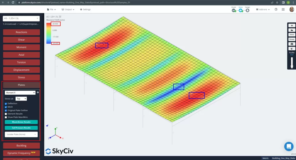
Abbildung 13. Momente in X-Richtung. (Strukturelles 3D, SkyCiv Cloud Engineering).
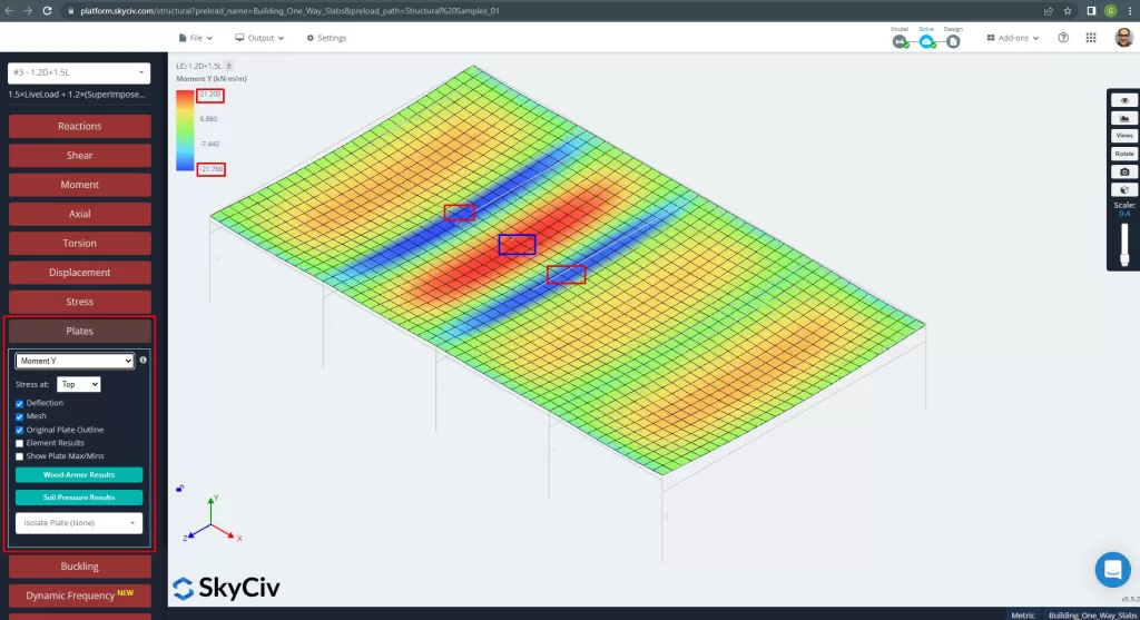
Abbildung 14. Momente in Y-Richtung. (Strukturelles 3D, SkyCiv Cloud Engineering).
Die lokalen Achsen der Plattenelemente sind unten angegeben.
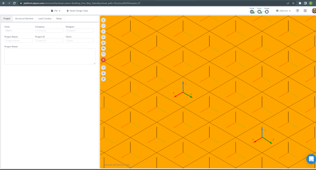
Abbildung 15. Lokale Plattenachsen. (Strukturelles 3D, SkyCiv Cloud Engineering).
Weitere Informationen zur automatisierten Bewehrungsplattenkonstruktion, siehe unsere Dokumentation Platten in SkyCiv.
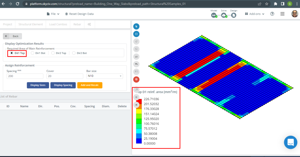
Abbildung 16. Obere D1-Verstärkung. (Strukturelles 3D, SkyCiv Cloud Engineering).
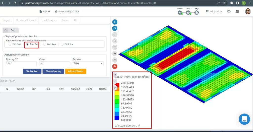
Abbildung 17. Untere D1-Verstärkung. (Strukturelles 3D, SkyCiv Cloud Engineering).
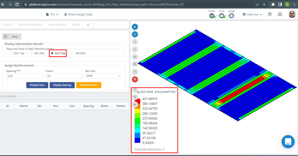
Abbildung 18. Obere D2-Verstärkung. (Strukturelles 3D, SkyCiv Cloud Engineering).
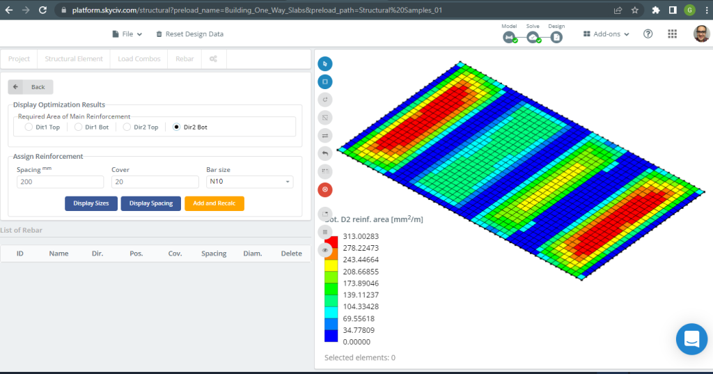
Abbildung 19. Untere D2-Verstärkung. (Strukturelles 3D, SkyCiv Cloud Engineering).
Ergebnisvergleich
Der letzte Schritt in diesem Beispiel für eine einseitige Deckenkonstruktion ist der Vergleich der durch die S3D-Analyse erhaltenen Stahlbewehrungsfläche (lokale Achsen “2”) und Handberechnungen.
| Momente und Stahlbereich | Äußere negative Linke | Äußerlich positiv | Äußeres negatives Recht | Innere negative Linke | Innen positiv | Inneres negatives Recht |
|---|---|---|---|---|---|---|
| \(EIN_{st, HandCalcs} {mm^2}\) | 334.82 | 436.31 | 481.099 | 481.099 | 334.8214 | 436.3100 |
| \(EIN_{st, S3D} {mm^2}\) | 285.13 | 313.00 | 427.69 | 427.69 | 313.00 | 427.69 |
| \(\Delta_{diff}\) (%) | 14.84 | 28.262 | 11.101 | 11.101 | 6.517 | 1.986 |
Wir können sehen, dass die Ergebnisse der Werte sehr nahe beieinander liegen. Dies bedeutet, dass die Berechnungen korrekt sind!
Beispiel für ein zweiseitiges Plattendesign
In diesem Abschnitt, Wir werden ein Beispiel entwickeln, das aus einem Grillsystem besteht.
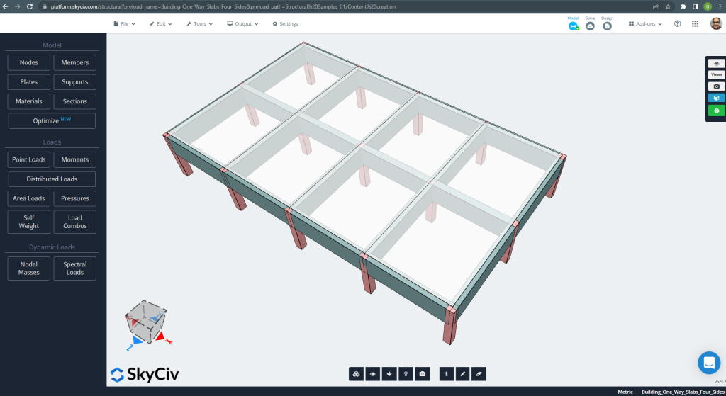
Abbildung 20. Grillsystem. (Strukturelles 3D, SkyCiv Cloud Engineering).
Die Planmaße werden nachfolgend angezeigt
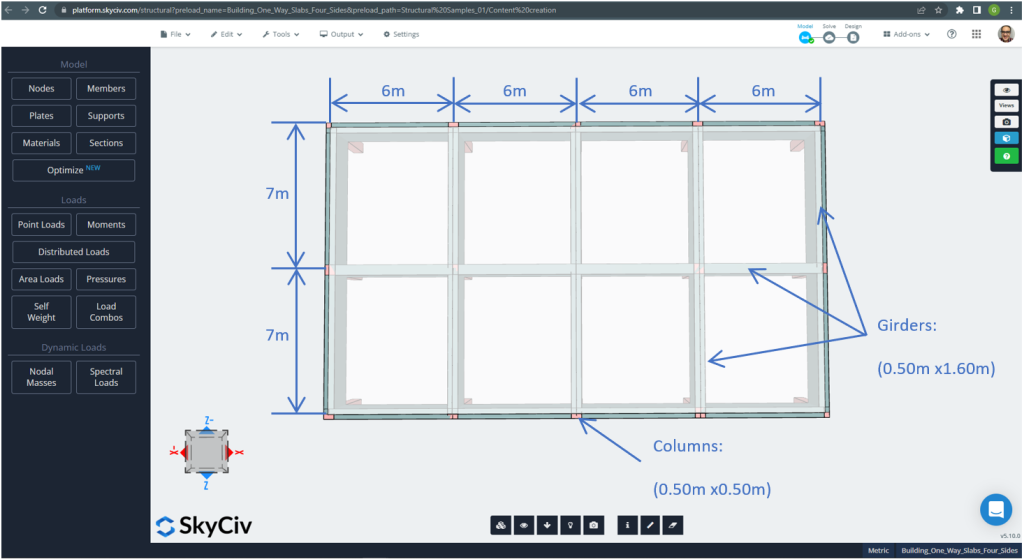
Abbildung 21. Planen Sie die Abmessungen für das Beispiel einer vierseitig verlaufenden Platte. (Strukturelles 3D, SkyCiv Cloud Engineering).
Für das Plattenbeispiel, Zusammenfassend, das Material, Elementeigenschaften, und jede Menge zu bedenken :
- Klassifizierung des Plattentyps: Zwei – Art und Weise Verhalten \(\frac{L_2}{L_1} \das 2 ; \frac{7 Mio.}{6 Mio.}=1,167 < 2.00 \) OK!
- Gebäudebesetzung: Wohnnutzung
- Plattendicke \(t_{Platte}=0.25m\)
- Stahlbetondichte unter der Annahme eines Stahlverstärkungsverhältnisses von 0.5% \(\rho_w = 24 \frac{kN}{m^3} + 0.6 \frac{kN}{m^3} \mal 0.5 = 24.3 \frac{kN}{m^3} \)
- Charakteristische Betondruckfestigkeit bei 28 Tage \(f’c = 25 MPa \)
- Konkreter Elastizitätsmodul nach australischem Standard \(E_c = 26700 MPa \)
- Eigengewicht der Platte \(Dead = \rho_w \times t_{Platte} = 24.3 \frac{kN}{m^3} \mal 0,25m = 6.075 \frac {kN}{m^2}\)
- Überlagerte Eigenlast \(SD = 3.0 \frac {kN}{m^2}\)
- Live-Last \(L = 2.0 \frac {kN}{m^2}\)
Handberechnung nach AS3600-Standard
In diesem Abschnitt, Wir berechnen den erforderlichen Bewehrungsstahl anhand der Referenz des australischen Standards. Wir ermitteln zunächst das gesamte faktorisierte Biegemoment, das von den einheitlichen Breitenstreifen der Platte in jeder Biegehauptrichtung ausgeübt werden muss.
- Eigengewicht, \(g = (3.0 + 6.075) \frac{kN}{m^2} \mal 1 m = 9.075 \frac{kN}{ Mio.}\)
- Live-Last, \(q = (2.0) \frac{kN}{m^2} \mal 1 m = 2.0 \frac{kN}{ Mio.}\)
- Grenzlast, \(Fd = 1.2\times g + 1.5\mal q = (1.2\mal 9.075 + 1.5\mal 2.0)\frac{kN}{ Mio.} =13.89 \frac{kN}{ Mio.} \)
Bemessungsmomente und Koeffizienten
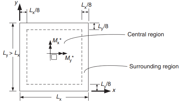
Abbildung 22. Ausrichtung einer Zwei-Wege-Platte zur Bestimmung positiver Momente. (Yew-Chaye Loo & Sanual Hug Chowdhury , “Bewehrter und vorgespannter Beton”, 22. Auflage, Cambridge University Press)
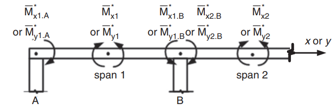
Abbildung 23. Bestimmung negativer Momente in einer Zwei-Wege-Platte. (Yew-Chaye Loo & Sanual Hug Chowdhury , “Bewehrter und vorgespannter Beton”, 22. Auflage, Cambridge University Press)
| Kantenzustand | Kurzspannenkoeffizienten (\(\beta_x\)) | Langzeitkoeffizienten (\(\beta_y)\) alle Werte von \(\frac{L_y}{L_x}\) | |||||||
|---|---|---|---|---|---|---|---|---|---|
| Werte von \(\frac{L_y}{L_x}\) | |||||||||
| 1.0 | 1.1 | 1.2 | 1.3 | 1.4 | 1.5 | 1.75 | \(\Die Hälfte der Wandhöhe von der Unterseite der Basis für den Fall des 2.0\) | ||
| 1. Vier Kanten durchgehend | 0.024 | 0.028 | 0.032 | 0.035 | 0.037 | 0.040 | 0.044 | 0.048 | 0.024 |
| 2. Eine kurze Kante diskontinuierlich | 0.028 | 0.032 | 0.036 | 0.038 | 0.041 | 0.043 | 0.047 | 0.050 | 0.028 |
| 3. Eine lange Kante unterbrochen | 0.028 | 0.035 | 0.041 | 0.046 | 0.050 | 0.054 | 0.061 | 0.066 | 0.028 |
| 4. Zwei kurze Kanten unterbrochen | 0.034 | 0.038 | 0.040 | 0.043 | 0.045 | 0.047 | 0.050 | 0.053 | 0.034 |
| 5. Zwei lange Kanten unterbrochen | 0.034 | 0.046 | 0.056 | 0.065 | 0.072 | 0.078 | 0.091 | 0.100 | 0.034 |
| 6. Zwei benachbarte Kanten diskontinuierlich | 0.035 | 0.041 | 0.046 | 0.051 | 0.055 | 0.058 | 0.065 | 0.070 | 0.035 |
| 7. Drei Kanten diskontinuierlich (eine lange Kante durchgehend) | 0.043 | 0.049 | 0.053 | 0.057 | 0.061 | 0.064 | 0.069 | 0.074 | 0.043 |
| 8. Drei Kanten diskontinuierlich (eine kurze Kante durchgehend) | 0.043 | 0.054 | 0.064 | 0.072 | 0.078 | 0.084 | 0.096 | 0.105 | 0.043 |
| 9. Vier Kanten diskontinuierlich | 0.056 | 0.066 | 0.074 | 0.081 | 0.087 | 0.093 | 0.103 | 0.111 | 0.056 |
Tabelle 1. (Yew-Chaye Loo & Sanual Hug Chowdhury , “Bewehrter und vorgespannter Beton”, 22. Auflage, Cambridge University Press)
Das folgende Bild erläutert alle neun Fälle, auf die sich die obige Tabelle bezieht
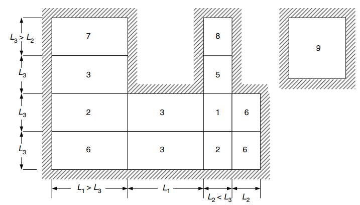
Abbildung 24. Randbedingungen für zweiseitig gelagerte Decken. (Yew-Chaye Loo & Sanual Hug Chowdhury , “Bewehrter und vorgespannter Beton”, 22. Auflage, Cambridge University Press)
Designmomente für die Zentralregion (Fall 6 Zwei benachbarte Kanten diskontinuierlich) :
- \(L_x = 6m, L_y=7m, \frac{L_y}{L_x} = frac{7 Mio.}{6 Mio.}= 1.167 \) Werte, die linear interpoliert werden sollen
- Positiv:
- \(M_x = {\beta_x}{F_d}{L_x^2} = {0.04435}\mal {13.89 \frac{kN}{ Mio.}}\mal{(6 Mio.)^ 2}=22.177 kNm\)
- \(M_y = {\beta_y}{F_d}{L_x^2} ={0.035}\mal {13.89 \frac{kN}{ Mio.}}\mal{(6 Mio.)^ 2}=17,501 kNm \)
- Negative Außenspanne:
- \(M_{x1,A} = -\lambda_e \times M_x = -0.5 \mal 22.177 kNm = – 11.089 kNm\)
- \(M_{y1,A} = -\lambda_e \times M_y = -0.5 \mal 17.501 kNm = -8.751 kNm \)
- Negative Innenspanne:
- \(M_{x1, B} = -\lambda_{1x} \mal M_x = -1.33 \mal 22.177 kNm = – 29.495 kNm\)
- \(M_{y1, B.} = -\lambda_{1j} \mal M_y = -1.33 \mal 17.501 kNm = -23.276 kNm \)
Designmomente für die Zentralregion (Fall 3 Eine lange Kante unterbrochen) :
- \(L_x = 6m, L_y=7m, \frac{L_y}{L_x} = frac{7 Mio.}{6 Mio.}= 1.167 \) Werte, die linear interpoliert werden sollen
- Positiv:
- \(M_x = {\beta_x}{F_d}{L_x^2} = {0.03902}\mal {13.89 \frac{kN}{ Mio.}}\mal{(6 Mio.)^ 2}= 19.512 kNm\)
- \(M_y = {\beta_y}{F_d}{L_x^2} ={0.028}\mal {13.89 \frac{kN}{ Mio.}}\mal{(6 Mio.)^ 2}= 14.001 kNm \)
- Negative Innenspanne:
- \(M_{x1, B} = -\lambda_{1x} \mal M_x = -1.33 \mal 19.512 kNm = – 25.951 kNm\)
- \(M_{y1, B} = -\lambda_{1j} \mal M_y = -1.33 \mal 14.001 kNm = – 18.621 kNm \)
- Negative im zweiten Abschnitt:
- \(M_{x2,B} = -\lambda_{2x} \mal M_x = -1.33 \mal 19.512 kNm = – 25.951 kNm\)
- \(M_{y2,B} = -\lambda_{2j} \mal M_y = -1.33 \mal 14.001 kNm = – 18.621 kNm \)
Bewehrungsstahl für X-Richtung
| \(\Alpha) und Momente | Äußere negative Linke | Äußerlich positiv | Äußeres negatives Recht | Innere negative Linke | Innen positiv | Inneres negatives Recht |
|---|---|---|---|---|---|---|
| M-Wert | 11.089 | 22.177 | 29.495 | 25.951 | 19.512 | 25.951 |
| \(\rho_t\) | 0.00055614 | 0.00112 | 0.001496 | 0.001313 | 0.000984 | 0.001313 |
| Zu | 0.015395 | 0.0310 | 0.0414 | 0.0364 | 0.0272 | 0.0364 |
| \(\Phi) | 0.8 | 0.8 | 0.8 | 0.8 | 0.8 | 0.8 |
| \(EIN_{st} {mm^2}\) | 334.8214 | 334.8214 | 335.08233 | 334.821 | 334.8214 | 334.8214 |
Bewehrungsstahl für Y-Richtung
| \(\Alpha) und Momente | Äußere negative Linke | Äußerlich positiv | Äußeres negatives Recht | Innere negative Linke | Innen positiv | Inneres negatives Recht |
|---|---|---|---|---|---|---|
| M-Wert | 8.751 | 17.501 | 23.276 | 18.621 | 14.001 | 18.621 |
| \(\rho_t\) | 0.0004383 | 0.0008811 | 0.001176 | 0.0009381 | 0.000703 | 0.0009381 |
| Zu | 0.0121 | 0.0244 | 0.03256 | 0.02597 | 0.0195 | 0.02597 |
| \(\Phi) | 0.8 | 0.8 | 0.8 | 0.8 | 0.8 | 0.8 |
| \(EIN_{st} {mm^2}\) | 334.821 | 334.821 | 334.821 | 334.821 | 334.8214 | 334.821 |
Wenn Sie neu bei SkyCiv sind, Melden Sie sich an und testen Sie die Software selbst!
Ergebnisse des SkyCiv S3D Plate Design-Moduls
Nach der Verfeinerung des Modells, Es ist an der Zeit, eine lineare elastische Analyse durchzuführen.
Beim Entwerfen von Platten, Wir müssen prüfen, ob die vertikale Verschiebung kleiner als das vom Code zulässige Maximum ist. Australische Standards haben eine maximale vertikale Verschiebung der Wartungsfreundlichkeit festgelegt \(\frac{L.}{250}= frac{6000mm}{250}=24.0 mm\).
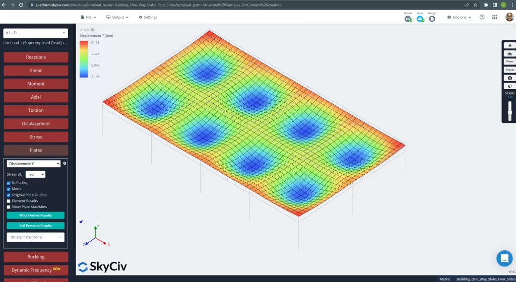
Abbildung 25. Vertikale Verschiebung im Grillplattensystem. (Strukturelles 3D, SkyCiv Cloud Engineering).
Das Bild oben zeigt uns die vertikale Verschiebung. Der Maximalwert beträgt -1,179 mm und liegt damit unter dem maximal zulässigen Wert von -24 mm. Deshalb, Die Steifigkeit der Platte ist ausreichend.
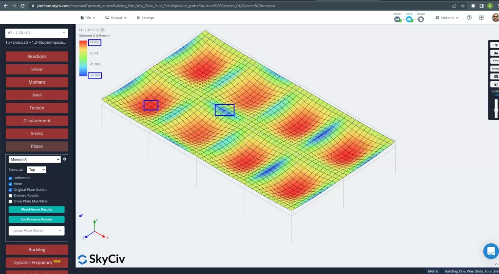
Abbildung 26. Plattenmomente in X-Richtung. (Strukturelles 3D, SkyCiv Cloud Engineering).
Bilder 27 und 28 bestehen aus dem Biegemoment in jeder Hauptrichtung. Nehmen Sie die Momentenverteilung und -werte, die Software, SkyCiv, kann dann die gesamte Stahlbewehrungsfläche erhalten.
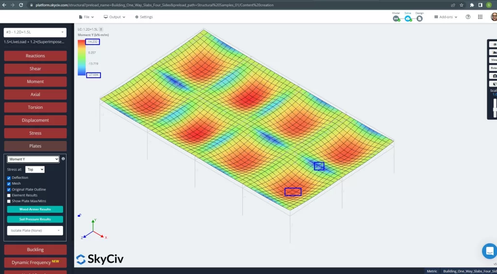
Abbildung 27. Plattenmomente in Y-Richtung. (Strukturelles 3D, SkyCiv Cloud Engineering).
Stahlverstärkungsbereiche:
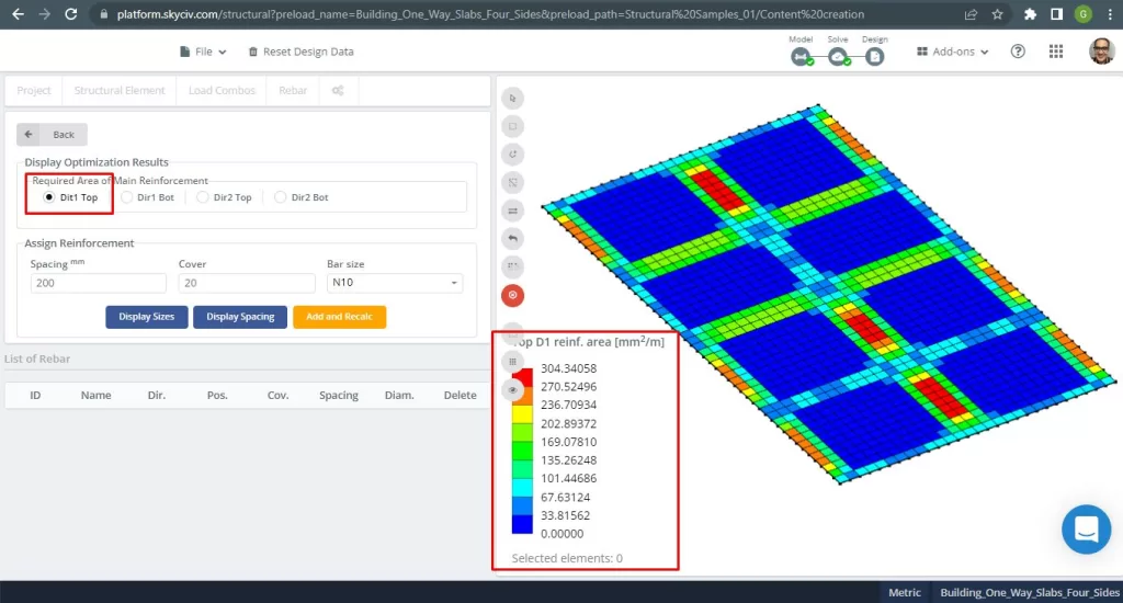
Abbildung 28. Obere Stahlbewehrungsbewehrung in Richtung 1. (Strukturelles 3D, SkyCiv Cloud Engineering).
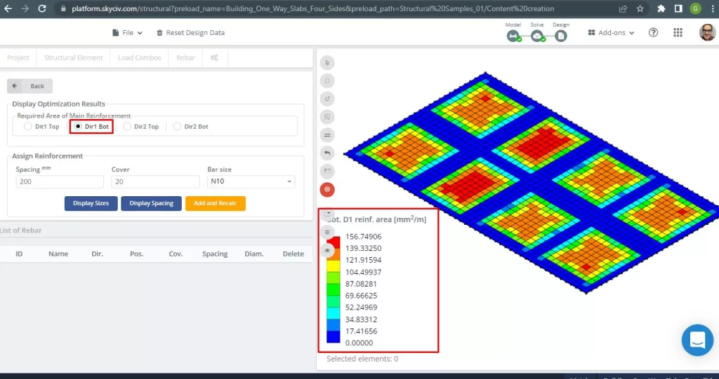
Abbildung 29. Untere Stahlbewehrungsbewehrung in Richtung 1. (Strukturelles 3D, SkyCiv Cloud Engineering).
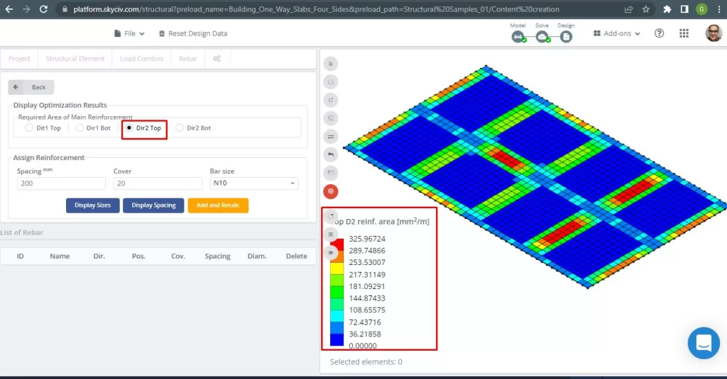
Abbildung 30. Obere Stahlbewehrungsbewehrung in Richtung 2. (Strukturelles 3D, SkyCiv Cloud Engineering).
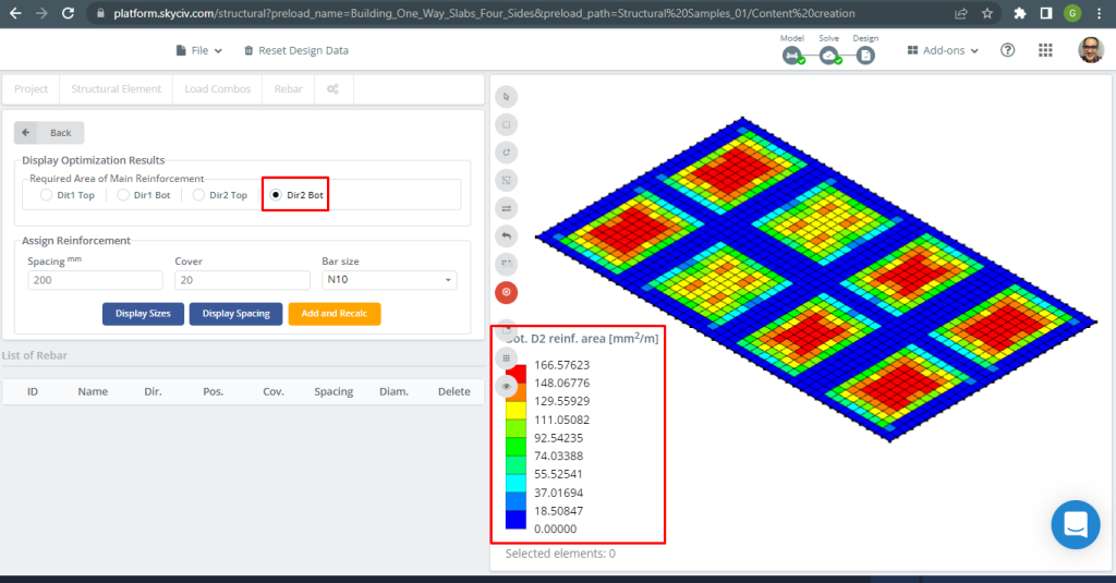
Abbildung 31. Untere Stahlbewehrungsbewehrung in Richtung 2. (Strukturelles 3D, SkyCiv Cloud Engineering).
Ergebnisvergleich
Der letzte Schritt in diesem Beispiel für eine einseitige Deckenkonstruktion ist der Vergleich der Stahlbewehrungsfläche, die durch S3D-Analyse und Handberechnungen ermittelt wurde.
Bewehrungsstahl für X-Richtung
| Momente und Stahlbereich | Äußere negative Linke | Äußerlich positiv | Äußeres negatives Recht | Innere negative Linke | Innen positiv | Inneres negatives Recht |
|---|---|---|---|---|---|---|
| \(EIN_{st, HandCalcs} {mm^2}\) | 334.8214 | 334.8214 | 335.08233 | 334.821 | 334.8214 | 334.8214 |
| \(EIN_{st, S3D} {mm^2}\) | 289.75 | 149.35 | 325.967 | 325.967 | 116.16 | 217.311 |
| \(\Delta_{diff}\) (%) | 13.461 | 55.39 | 2.720 | 2.644 | 65.307 | 35.0964 |
Bewehrungsstahl für Y-Richtung
| Momente und Stahlbereich | Äußere negative Linke | Äußerlich positiv | Äußeres negatives Recht | Innere negative Linke | Innen positiv | Inneres negatives Recht |
|---|---|---|---|---|---|---|
| \(EIN_{st, HandCalcs} {mm^2}\) | 334.821 | 334.821 | 334.821 | 334.821 | 334.821 | 334.821 |
| \(EIN_{st, S3D} {mm^2}\) | 270.524 | 156.75 | 304.34 | 304.34 | 156.75 | 270.52 |
| \(\Delta_{diff}\) (%) | 19.203 | 53.184 | 9.104 | 9.104 | 53.184 | 19.204 |
Der Unterschied ist bei positiven Momenten etwas hoch und der Grund wäre das Vorhandensein von Trägern mit hoher Torsionssteifigkeit, die sich auf die Ergebnisse der Platten-Finite-Elemente-Analyse und die Berechnungen für die Biegung von Bewehrungsstahl auswirken.
Wenn Sie neu bei SkyCiv sind, Melden Sie sich an und testen Sie die Software selbst!
Verweise
- Yew-Chaye Loo & Sanual Hug Chowdhury , “Bewehrter und vorgespannter Beton”, 22. Auflage, Cambridge University Press.
- Bazan Enrique & Meli Piralla, “Seismisches Design von Bauwerken”, 1ed, KLAR.
- Australisches Handbuch für Bauingenieure, Australisches Handbuch für Bauingenieure, AS 3600:2018