Basisplatten -Design -Beispiel mit eN 1993-1-8-2005, IM 1993-1-1-2005 und EN 1992-1-1-2004
Problemanweisung
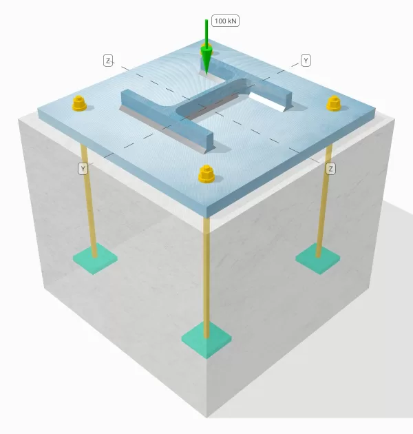
Bestimmen Sie, ob die ausgestaltete Säule-zu-Base-Plattenverbindung für eine 100-kn-Komprimierungslast ausreicht.
Gegebene Daten
Spalte:
Spaltenabschnitt: ER 200 B.
Säulenbereich: 7808 mm2
Säulenmaterial: S235
Grundplatte:
Grundplattenabmessungen: 400 mmx 400 mm
Grundplattendicke: 20 mm
Grundplattenmaterial: S235
Fugenmörtel:
Fugenmörtel Dicke: 20 mm
Beton:
Konkrete Abmessungen: 450 mmx 450 mm
Betondicke: 380 mm
Betonmaterial: C20/25
Schweißnähte:
Drucklast nur durch Schweißnähte übertragen? NEIN
Modell im kostenlosen SkyCiv-Tool
Modellieren Sie noch heute das oben stehende Grundplattendesign mit unserem kostenlosen Online-Tool! Keine Anmeldung erforderlich.
Schritt-für-Schritt-Berechnungen
Prüfen #1: Berechnen Sie die Schweißkapazität
Da die Kompressionslast nicht allein durch Schweißnähte übertragen wird, Eine ordnungsgemäße Kontaktlagerfläche ist erforderlich, um sicherzustellen, dass die Last über das Lager übertragen wird. Beziehen sich auf IM 1090-2:2018 Klausel 6.8 Für die Kontaktlagervorbereitung.
zusätzlich, Verwenden Sie eine minimale Schweißnahtgröße spezifiziert im Eurocode.
Prüfen #2: Berechnen Sie die Tragfähigkeit des Betons und die Streckgrenze der Bodenplatte
Der erste Schritt besteht darin, die konstruktive Druckfestigkeit der Verbindung zu bestimmen, was von der Geometrie des Trägers abhängt (Beton) und die Geometrie der belasteten Fläche (Grundplatte).
Wir beginnen mit der Berechnung des Alpha-Faktors, Dies erklärt die Diffusion der konzentrierten Kraft innerhalb des Fundaments.
Gemäß IM 1992-1-1:2004, Klausel 6.7, Der Alpha-Koeffizient ist das Verhältnis der belasteten Fläche zur maximalen Verteilungsfläche, die eine ähnliche Form wie die belastete Fläche hat.
Wir verwenden die Gleichung von Teil 6.1 Teil: mehrstöckige Stahlbauten 5 durch Arcelor Mittal, Peiner Träger, und Corus um den Alpha-Faktor zu berechnen.
\(
\alpha = min left(
1 + \frac{t_{\Text{konz}}}{\max(L_{\Text{bp}}, B_{\Text{bp}})},
1 + 2 \links( \frac{e_h}{L_{\Text{bp}}} \richtig),
1 + 2 \links( \frac{e_b}{B_{\Text{bp}}} \richtig),
3
\richtig)
\)
\(
\alpha = min left(
1 + \frac{380 \, \Text{mm}}{\max(400 \, \Text{mm}, 400 \, \Text{mm})},
1 + 2 \links( \frac{25 \, \Text{mm}}{400 \, \Text{mm}} \richtig),
1 + 2 \links( \frac{25 \, \Text{mm}}{400 \, \Text{mm}} \richtig),
3
\richtig)
\)
\(
\Alpha = 1.125
\)
wo,
\(
e_h = frac{L_{\Text{konz}} – L_{\Text{bp}}}{2} = frac{450 \, \Text{mm} – 400 \, \Text{mm}}{2} = 25 \, \Text{mm}
\)
\(
e_b = frac{B_{\Text{konz}} – B_{\Text{bp}}}{2} = frac{450 \, \Text{mm} – 400 \, \Text{mm}}{2} = 25 \, \Text{mm}
\)
Sobald die Geometrie definiert ist, Anschließend ermitteln wir die Druckfestigkeit des Betons IM 1992-1-1:2004, Gl. 3.15.
\(
f_{CD} = frac{\= Abstand des Abschnitts, in dem die Scherung berücksichtigt wird, zur Fläche des nächsten Auflagers{cc} f_{ck}}{\Gamma_c} = frac{1 \mal 20 \, \Text{MPa}}{1.5} = 13.333 \, \Text{MPa}
\)
Als nächstes, Wir gehen von einem Wert für den Beta-Koeffizienten aus. Da Fugenmörtel vorhanden ist, Beta-Wert kann sein 2/3. Wir berechnen die Bemessungstragfestigkeit der Verbindung anhand der kombinierten Formeln von IM 1993-1-8:2005 Gl. 6.6, und IM 1992-1-1:2004 Gl. 6.63.
\(
f_{jd} = beta alpha f_{CD} = 0.66667 \mal 1.125 \mal 13.333 \, \Text{MPa} = 10 \, \Text{MPa}
\)
Im zweiten Teil geht es um die Berechnung der Tragfähigkeit der Grundplatte.
Da uns die Bemessungstragfähigkeit der Verbindung bereits vorliegt, Damit ermitteln wir den kleinsten Auskragabstand der Grundplatte, der die volle Traglast erfährt. Wir beziehen uns auf die SCI P358 Beispiel auf Seite 243 und IM 1993-1-1:2005 Klausel 6.2.5.
\(
c = t_{\Text{bp}} \sqrt{\frac{f_{y_{\Text{bp}}}}{3 f_{jd} \Um es zu berechnen{M0}}} = 20 \, \Text{mm} \mal sqrt{\frac{225 \, \Text{MPa}}{3 \mal 10 \, \Text{MPa} \mal 1}} = 54.772 \, \Text{mm}
\)
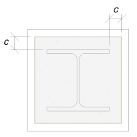
Wir werden dieses Maß verwenden, um die effektive Fläche der Grundplatte zu berechnen. Das „c’ Das von uns berechnete Maß kann sich in der Nähe des Flansches überlappen oder nicht überlappen. Wenn es sich überschneidet, Wir gehen davon aus, dass es sich bei dem Abschnitt um einen rechteckigen Abschnitt handelt. Wenn es nicht überlappt, Wir nehmen die Form der Säule an.
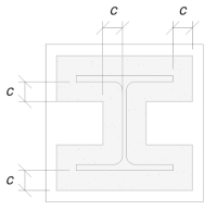
Ohne Überlappung
Mit Überlappung
Wir haben festgestellt, dass das „c’ Die Dimension überschneidet sich nicht. Deshalb, mit SCI P358 S. 243, Die wirksame Fläche beträgt:
\(
A_e = 4c^2 + P_{\Text{col}}c + EIN_{\Text{col}} = 4 \mal 54,772^2 \, \Text{mm}^ 2 + 1182 \, \Text{mm} \mal 54.772 \, \Text{mm} + 7808 \, \Text{mm}^2 = 84549 \, \Text{mm}^ 2
\)
Dabei ist zu beachten, dass die Nutzfläche nicht kleiner als die Grundplattenfläche sein sollte.
Schließlich, wir werden verwenden IM 1993-1-8:2005 Gl. 6.6, und EN 1992-1-1:2004, Gl. 6.63 zur Berechnung der Bemessungstragfähigkeit der Grundplattenverbindung.
\(
N_{Rd} = left( \Min.(A_e, A_0) \richtig) f_{jd} = left( \Min.(84549 \, \Text{mm}^ 2, 160000 \, \Text{mm}^ 2) \richtig) \mal 10 \, \Text{MPa} = 845.49 \, \Text{kN}
\)
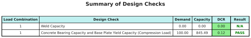
Schon seit 845.49 kN > 100 kN, Das Design ist ausreichend!
Entwurfszusammenfassung
Die Skyciv-Basisplattentwurfsoftware kann automatisch einen schrittweisen Berechnungsbericht für dieses Entwurfsbeispiel erstellen. Es enthält auch eine Zusammenfassung der durchgeführten Schecks und deren resultierenden Verhältnisse, Die Informationen auf einen Blick leicht zu verstehen machen. Im Folgenden finden Sie eine Stichprobenzusammenfassungstabelle, Welches ist im Bericht enthalten.
SKYCIV -Beispielbericht
Sehen Sie sich den Detaillierungsgrad und die Klarheit an, die Sie von einem SkyCiv-Grundplatten-Designbericht erwarten können. Der Bericht umfasst alle wichtigen Designprüfungen, Gleichungen, und Ergebnisse werden in einem klaren und leicht lesbaren Format präsentiert. Es entspricht vollständig den Designstandards. Klicken Sie unten, um einen Beispielbericht anzuzeigen, der mit dem SkyCiv-Grundplattenrechner erstellt wurde.
Basisplattensoftware kaufen
Kaufen Sie die Vollversion des Basisplatten -Designmoduls selbst ohne andere Skyciv -Module selbst. Auf diese Weise erhalten Sie einen vollständigen Satz von Ergebnissen für die Basisplattendesign, Einbeziehung detaillierter Berichte und mehr Funktionen.