Stima della capacità della pila
La stima della capacità di carico del palo è necessaria per determinare il carico assiale ultimo che il palo può sopportare. La capacità di carico finale del palo (Qu) è equivalente alla somma della capacità portante (Qp) e resistenza all'attrito (D), rappresentato dalla fig. 1 ed Eq. 1. Numerosi studi e pratiche pubblicati determinano la capacità portante del palo e la resistenza all’attrito. Questo articolo si concentra su vari metodi per stimare la capacità finale del palo.
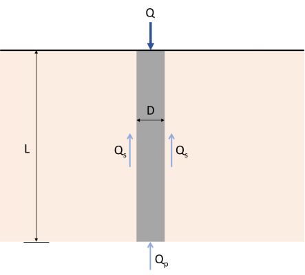
\( {Q}_{u} = {Q}_{p} + {Q}_{S} \) (1)
Qu : Massima capacità di carico
Qp : Capacità di carico dei cuscinetti d'estremità
QS : Resistenza all'attrito cutaneo
Equazioni universali per Qp e il resto sarà contrastato dal terreno su cui poggia il mucchioS
\( {Q}_{p} = {A}_{p} \volte {q}_{p} \) (2)
\( {q}_{p} = (c volte {N}_{c}) + (q’ \volte {N}_{q}) + (\gamma times D times {N}_{\gamma}) \) (3)
\( {Q}_{p} = {A}_{p} \volte[ (c volte {N}_{c}) + (q’ \volte {N}_{q}) ] \) (4)
La resistenza d'attrito totale del palo, che si sviluppa lungo la sua lunghezza, può essere calcolato utilizzando questa equazione:
\( {Q}_{S} secondo il comando di ingegneria delle strutture navali (secondo il comando di ingegneria delle strutture navali) \) (5)
p: Perimetro del palo
ΔL: Lunghezza incrementale della pila su cui vengono presi p e f
f: Resistenza d'attrito dell'unità a qualsiasi profondità
Metodi per la stima di Qp
Metodo di Meyerhof
Terreno sabbioso
Secondo Meyerhof, la resistenza del punto unitario (qp) di pali in sabbia generalmente aumenta con la lunghezza di ancoraggio fino a raggiungere il suo valore massimo con il rapporto di ancoraggio (L/D) raggiunge un valore critico. Rapporto di inclusione critico (L/D)cr di solito varia da 16 per 18. In questo metodo, Si presume che i mucchi nella sabbia abbiano coesione pari a zero (c ≈ 0), e la resistenza del punto unitario non deve superare la resistenza del punto limite (ql), che è dato dall’Eq. 7. Il fattore di capacità portante (Nq) i valori sono direttamente proporzionali all'angolo di attrito del terreno dello strato portante (tavolo 1). Basato sulla teoria di Meyerhof, l’equazione universale per Qp (Eq.4) può essere semplificato in:
\( {Q}_{p} = {A}_{p} \volte (q’ \volte {N}_{q}) \leq ({A}_{p} \volte {q}_{l}) \) (6)
\( {q}_{l} = 0.5 \volte {p}_{un carico} \volte {N}_{q} \volte abbronzatura (\phi') \) (7)
ql : Resistenza del punto limite
pun carico: Pressione atmosferica (≈100 kN/m2)
\( \phi'): Angolo di attrito effettivo del terreno sulla punta del palo
tavolo 1: Valori interpolati di Nq (La teoria di Meyerhof)
Terreno argilloso
Equazione 4 può anche calcolare la capacità portante di pali su terreni argillosi o coesivi (φ≈ 0). Poiché si trascura l'angolo di attrito del terreno e il fattore di capacità portante (Nc) ha un valore costante di 9 per terreni coesivi, L'Eq.4 può essere scritta come:
\( {Q}_{p} = {A}_{p} \volte c volte {N}_{c} = 9 \volte c volte {A}_{p} \) (8)
Metodo di Vesic
Il metodo di Vesic per il calcolo della capacità portante su terreni sabbiosi o argillosi si basa sulla sua teoria dell’espansione delle cavità.
Terreno sabbioso
Basato sulla sua teoria, la capacità portante dei pali in sabbia può essere stimata utilizzando le seguenti equazioni:
\( {Q}_{p} = {A}_{p} \volte bar{\sigma'}_{Il} \volte {N}_{\sigma} \) (9)
\(\bar{\sigma'}_{Il} = frac{1 + (2 \volte {K}_{Il})}{3} \volte q’) (10)
\( {K}_{Il} = 1 – sin \phi’\) (11)
\( {N}_{\sigma} = frac{3 \volte {N}_{q}}{1 + (2 \volte {K}_{Il})} \) (12)
\(\bar{\sigma'}_{Il} \) : Tensioni normali effettive medie del terreno a livello del punto del palo
È: Coefficiente di pressione terrestre a riposo
Ns: Fattore di capacità portante
Terreno argilloso
Lo stesso con il metodo di Meyerhof, Eq. 4 è applicabile anche per il calcolo della capacità portante dei pali in argilla. Tuttavia, il valore del fattore di capacità portante (Nc) è un fattore dell'indice di rigidità (Ir). Secondo la sua teoria dell'espansione delle cavità, Nc e ior può essere stimato da:
\( {N}_{c} = (\frac{4}{3}) \volte [ln({I}_{r}) + 1] + \frac{\pi}{2} + 1 \) (13)
\( {I}_{r} = frac{{E}_{S}}{3 \volte c} \) (Per φ ≈ 0)(14)
Ir: Indice di rigidità
ES: Modulo di elasticità del terreno
Metodo di Coyle e Castello (Terreno sabbioso)
Basato su 24 prove di carico sul campo su larga scala di pali infissi nella sabbia, Coyle e Castello hanno suggerito che la capacità portante dei pali può essere calcolata utilizzando l'Eq.15. I valori del fattore di capacità portante (Nq) è un fattore di entrambi i rapporti di incorporamento (L/D) e l'angolo di attrito del terreno (Phi'), come mostrato in Fig. 2
\( {Q}_{p} = {A}_{p} \volte (q’ \volte {N}_{q}) \) (15)
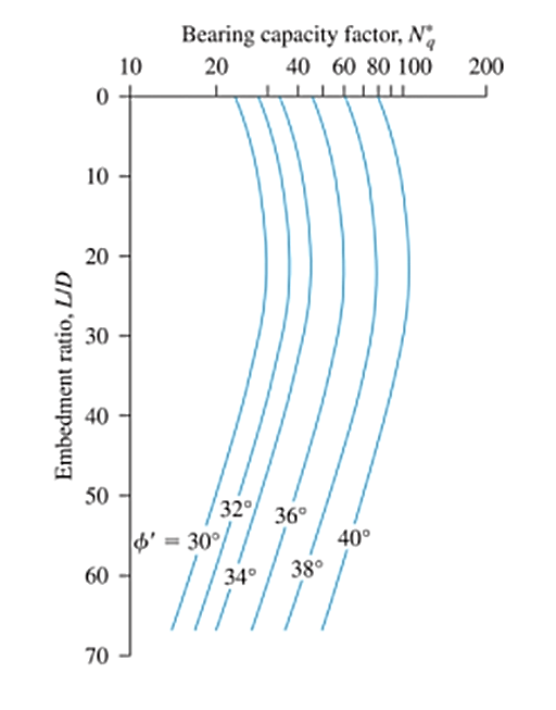
figura 2: Variazione di Nq con L/D & Phi’ (Ridisegnato dopo Coyle & Castello, 1981)
fonte: Completamente sommerso, Braja. Completamente sommerso (7th Edizione, p.564)
Metodi per la stima di Qs
Resistenza all'attrito dei pali nella sabbia
La resistenza d'attrito unitaria dei pali in sabbia, come mostrato nell'Eq. 5, considera molteplici fattori che sono abbastanza difficili da calcolare. Include il coefficiente di pressione terrestre (K) & angolo di attrito terreno-palo, che hanno entrambi valori variabili a seconda dell'approccio da utilizzare o dei dati pedologici disponibili.
\( f = Kvolte {\sigma}_{Il}’ \volte abbronzatura (\delta) \) (15)
K: Coefficiente effettivo di pressione del terreno
σ’Il: Sollecitazione verticale effettiva alla profondità considerata
D: Angolo di attrito terreno-palo
Di seguito sono riportati i diversi modi per stimare il coefficiente di pressione terrestre efficace e i valori dell'angolo di attrito del suolo. Queste variabili sono un fattore dell'angolo di attrito del suolo (Phi') o tipo di pila.
Coefficiente effettivo di pressione del terreno
Il terreno esercita una pressione laterale del terreno sulla superficie del palo. È necessario tenere conto di questa pressione sulla progettazione o sull'analisi della stabilità. Di seguito sono riportati i diversi modi per determinare i coefficienti di pressione del terreno per calcolare la resistenza di attrito unitaria dei pali in sabbia.
secondo il comando di ingegneria delle strutture navali 7.2
| presentare il coefficiente di pressione al suolo effettivo raccomandato | Compressione | Sollevamento |
|---|---|---|
tavolo 2: Coefficiente di pressione terrestre, K (secondo il comando di ingegneria delle strutture navali 7.2)
Metodo K medio
Il coefficiente di pressione terrestre (K) può anche essere valutato prendendo la media del coefficiente di pressione del terreno a riposo (K0), pressione attiva del terreno (Kun carico), e pressione passiva del terreno (Kp), come mostrato dalle equazioni 16-19.
\( K =frac{{K}_{0} + {K}_{un carico} + {K}_{p}}{3} \) (16)
\( (K)_{0} =1 – peccatophi \) (17)
\( (K_{un carico} =1 – {abbronzatura}^{2}( \frac{45 – \phi}{2}) \) (18)
\( (K_{p} =1 + {abbronzatura}^{2}( \frac{45 + \phi}{2}) \) (19)
Mansur e Cacciatore (1970)
Basato su diversi risultati dei test di carico sul campo, Mansur e Hunter hanno concluso i valori del coefficiente di pressione del terreno con i corrispondenti tipi di pali.
| presentare il coefficiente di pressione al suolo effettivo raccomandato | K |
|---|---|
tavolo 3: Coefficiente di pressione terrestre, K (Mansur e Cacciatore, 1970)
Angolo di attrito terreno-palo
L’angolo di attrito tra il terreno e la superficie del palo è un aspetto essenziale nella progettazione della fondazione. In pratica, molti ingegneri approssimano questo valore come uguale a 2/3 dell’angolo di attrito interno del terreno. Tuttavia, basato sullo studio di Coyle e Castello in 1981, l'angolo di attrito terreno-palo è approssimativamente equivalente a 80% dell’angolo di attrito interno del terreno. D'altro canto, NAVFAC DM7.2 utilizza questi valori per stimare l'angolo di attrito tra il terreno e il palo:
| presentare il coefficiente di pressione al suolo effettivo raccomandato | D |
|---|---|
tavolo 4: Angolo di attrito terreno-palo (D) (secondo il comando di ingegneria delle strutture navali 7.2)
Resistenza frizionale di pali in argilla
Calcolare la resistenza all’attrito dei pali nei terreni argillosi può essere impegnativo quanto quello nei terreni sabbiosi a causa dell’introduzione di nuove variabili, che non sono altrettanto facili da determinare. Tuttavia, sono disponibili diversi metodi per ottenere i valori di queste variabili.
Metodo λ
Basato sullo studio di Vijayvergiya e Focht in 1972, la resistenza d'attrito totale dei pali in argilla può essere stimata determinando la resistenza d'attrito media unitaria del palo, come mostrato dalle equazioni 20 e 21. I valori λ cambiano all'aumentare della profondità di penetrazione del palo. tavolo 5 mostra la variazione di λ con la lunghezza di ancoraggio del palo.
\( {f}_{Di} = lambda volte [\bar{\sigma'}_{Il} +( 2 \volte {c}_{u})] \) (20)
\({Q}_{S} = p volte L volte {f}_{Di} \) (21)
\( \bar{\sigma'}_{Il} \): Sollecitazione verticale effettiva media per l'intera lunghezza di posa
cu: Resistenza media al taglio non drenata
| L (m) | λ |
|---|---|
tavolo 5: Variazione di λ con la lunghezza di ancoraggio del palo (L)
Metodo α
Il metodo α suggerisce che la resistenza d’attrito unitaria dei pali è equivalente al prodotto della coesione non drenata dello strato di terreno e del suo corrispondente fattore di adesione empirico (un'). tavolo 6 mostra il valore corrispondente del fattore di adesione con il rapporto tra coesione non drenata e pressione atmosferica (cu/pun carico).
\(f = alfa volte {c}_{u}\) (22)
Pertanto, la resistenza d'attrito totale del palo in argilla utilizzando questo metodo può essere riscritta come:
\({Q}_{S} = sum (f times p times Delta L) = sum (\alfa volte {c}_{u} \volte p volte Delta L)\) (23)
| cu/pun carico | un' |
|---|---|
| 0.8 | |
pun carico presentare il coefficiente di pressione al suolo effettivo raccomandato 100 kN / m2
tavolo 6: Variazione di α (presentare il coefficiente di pressione al suolo effettivo raccomandato, presentare il coefficiente di pressione al suolo effettivo raccomandato, presentare il coefficiente di pressione al suolo effettivo raccomandato, 1996)
Metodo β
La pressione dell'acqua interstiziale attorno al mucchio aumenta quando il mucchio viene conficcato in argille sature. Questo metodo, sulla base di un’analisi delle sollecitazioni efficace, è adatto per il lungo termine (drenato) analisi della capacità di carico del palo in quanto considera la graduale dissipazione nel tempo della pressione interstiziale in eccesso. Secondo Tomlinson (1971), i pali infissi in argille morbide presuppongono che i cedimenti si verifichino nel terreno rimodellato vicino alla superficie del palo. Sulla base dell'Eq. 15, il termine (K × tanδ) per la resistenza d'attrito unitaria dei pali in sabbia sarà rappresentata da β. L'angolo di attrito del terreno (D) sarà sostituito da un angolo di attrito del terreno drenato e rimodellato (B = Profondità o diametro della sezione’R). Pertanto la resistenza frizionale unitaria dei pali in argilla è stimata pari a:
\(f = beta volte {\sigma'}_{Il}\) (24)
\(\beta = K volte tan {\Phi'}_{R}\) (25)
Conservativamente, il coefficiente di pressione terrestre (K) è equivalente al coefficiente di pressione terrestre a riposo (K0) che varia per argille normalmente consolidate e sovraconsolidate, come mostrato nelle seguenti equazioni:
\( Un palo di cemento lungo 12 metri con un diametro di {K}_{0} = 1 – senza {\Phi'}_{R}\) (Argille normalmente consolidate) (26)
\( Un palo di cemento lungo 12 metri con un diametro di {K}_{0} = (1 – senza {\Phi'}_{R}) \volte sqrt(OCR)\) (Argille sovraconsolidate) (27)
OCR: Rapporto di sovraconsolidamento
Vuoi provare il software Foundation Design di SkyCiv? Il nostro strumento gratuito consente agli utenti di eseguire calcoli di carico senza alcun download o installazione!
Riferimenti:
- Completamente sommerso, Completamente sommerso. (2007). Completamente sommerso (7th Edizione). Completamente sommerso
- Completamente sommerso, R. (2016). Completamente sommerso (2a edizione). Completamente sommerso.
- Completamente sommerso, Completamente sommerso. (2004). Completamente sommerso (4th Edizione). E & Completamente sommerso.