Sistemi di solai considerati dalla norma
Gli standard australiani stabiliscono i requisiti minimi per la progettazione delle solette in cemento armato, come i tipi unidirezionali e bidirezionali. Per quanto riguarda la configurazione in pianta e l'inclusione delle travi, le lastre possono anche essere suddivise in lastre appoggiate su quattro lati, sistemi di travi e solette, lastre piane, e piatti piani. Queste tipologie sono riassunte nelle seguenti immagini.
Semplifica la conformità della progettazione delle lastre australiane con l'avanzato di SkyCiv Esportare il rapporto di calcolo dettagliato da utilizzare come deliverable o in un pacchetto di calcolo. Provalo! Applica facilmente AS 3600 controlli per lastre e lamiere piane.
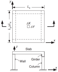
figura 1. Lastra appoggiata su quattro lati. (Yew-Chaye Loo & Sanual Abbraccio Chowdhury , “Cemento armato e precompresso”, 22a edizione, Cambridge University Press).
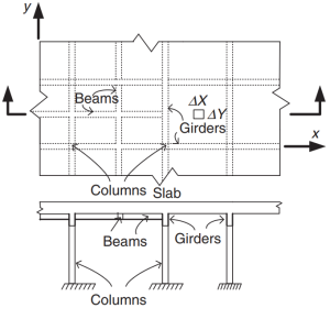
figura 2. Sistema di lastre di grigliatura. (Yew-Chaye Loo & Sanual Abbraccio Chowdhury , “Cemento armato e precompresso”, 22a edizione, Cambridge University Press).
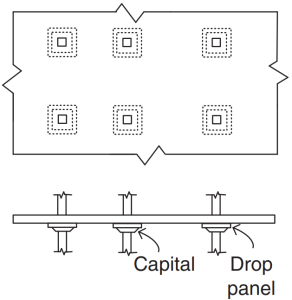
figura 3. Lastre piane. (Yew-Chaye Loo & Sanual Abbraccio Chowdhury , “Cemento armato e precompresso”, 22a edizione, Cambridge University Press).
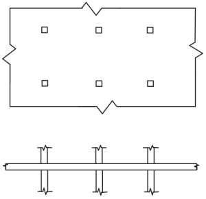
figura 4. Piatti Piani. (Yew-Chaye Loo & Sanual Abbraccio Chowdhury , “Cemento armato e precompresso”, 22a edizione, Cambridge University Press).
Lo Standard raccomanda alcuni metodi (procedure semplificate e collaudate) nella determinazione dei momenti flettenti:
- Clausola 6.10.2: Travi continue e solai unidirezionali
- Clausola 6.10.3: Lastre bidirezionali appoggiate su quattro lati
- Clausola 6.10.4: Solai bidirezionali a campate multiple
Lo scopo della norma è quello di progettare la quantità totale di armature in acciaio di armatura nelle direzioni principali nel sistema di solette. L'acciaio dell'armatura sarà calcolato per i momenti flettenti “Mx” e “Mio.” figura 5 mostra le altre forze o azioni in un elemento lastra finito in cui la norma prescrive i loro valori di resistenza.
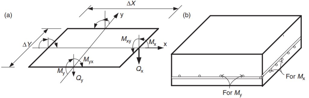
figura 5. Forze in un elemento solaio finito: momenti flettenti (Mx, Mio), momenti tortuosi (Mxy, Mix), e cesoie (Dx, Qy). (Yew-Chaye Loo & Sanual Abbraccio Chowdhury , “Cemento armato e precompresso”, 22a edizione, Cambridge University Press)
In questo articolo, svilupperemo due esempi di progettazione di lastre, sistemi di solette unidirezionali e bidirezionali, utilizzando le modalità semplificate orientate e consentite dal codice. In entrambi i casi, creeremo un modello SkyCiv S3D e confronteremo i risultati con i metodi sopra menzionati.
Se sei nuovo in SkyCiv, Iscriviti e testa tu stesso il software!
Esempio di progettazione di lastre unidirezionali
Di seguito è mostrato il piccolo edificio e le lastre che progetteremo
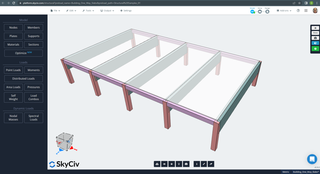
figura 6. Lastre unidirezionali in un piccolo esempio di edificio. (3D strutturale, Ingegneria del cloud SkyCiv).
Le dimensioni del piano sono riportate di seguito
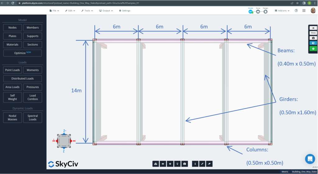
figura 7. Dimensioni in pianta ed elementi strutturali. (3D strutturale, Ingegneria del cloud SkyCiv).
Per l'esempio della lastra, In sintesi, il materiale, proprietà degli elementi, e carichi da considerare :
- Classificazione del tipo di soletta: Uno – modo di comportamento \(\frac{L_2}{L_1} > 2 ; \frac{14m}{6m}=2.33 > 2.00 \) Ok!
- Occupazione edilizia: Uso residenziale
- Spessore lastra \(t_{lastra}=0,25 m)
- Densità del cemento armato assumendo un rapporto di armatura in acciaio di 0.5% \(\ro_w = 24 \frac{kN}{m^3} + 0.6 \frac{kN}{m^3} \volte 0.5 = 24.3 \frac{kN}{m^3} \)
- Resistenza a compressione caratteristica del calcestruzzo a 28 giorni \(f'c = 25 MPa \)
- Modulo di elasticità del calcestruzzo secondo lo standard australiano \(E_c = 26700 MPa \)
- Peso proprio della lastra \(Dead = \rho_w \times t_{lastra} = 24.3 \frac{kN}{m^3} \volte 0,25 m = 6.075 \frac {kN}{m^2}\)
- Carico morto sovrapposto \(SD = 3.0 \frac {kN}{m^2}\)
- Carica in tempo reale \(L = 2.0 \frac {kN}{m^2}\)
Calcolo manuale secondo lo standard AS3600
In questa sezione, calcoleremo l'armatura in acciaio rinforzato richiesta utilizzando il riferimento dello standard australiano. Per prima cosa otteniamo il momento flettente totale fattorizzato che deve essere svolto dalla striscia di larghezza unitaria della soletta.
- Carico morto, \(g = (3.0 + 6.075) \frac{kN}{m^2} \volte 1 m = 9.075 \frac{kN}{m}\)
- Carica in tempo reale, \(q = (2.0) \frac{kN}{m^2} \volte 1 m = 2.0 \frac{kN}{m}\)
- Carico finale, \(Fd = 1.2\times g + 1.5\volte q = (1.2\volte 9.075 + 1.5\volte 2.0)\frac{kN}{m} =13.89 \frac{kN}{m} \)
Utilizzando il metodo semplificato specificato dalla norma, primo, è obbligatorio rispettare le seguenti restrizioni:
- \(\frac{L_i}{L_j} \il 1.2 . \frac{6m}{6m} =1 < 1.2 \). Ok!
- Il carico deve essere uniforme. Ok!
- \(q \le 2g. q=2 \frac{kN}{m} < 18.15 \frac{kN}{m}\). Ok!
- La sezione trasversale della soletta deve essere uniforme. Ok!.
Spessore minimo consigliato, d
\(d \ge \frac{L_{fe}}{{k_3}{k_4}{\sqrt[3]{\frac{\frac{\Delta}{L_{ef}}{E_c}}{F_{d, ef}}}}}\)
Dove
- \(k_3 = 1.0; k_4 = 1.75 \)
- \(\frac{\Delta}{L_{ef}}=1/250 \)
- \(E_c = 27600 MPa \)
- \(F_{d,ef} = (1.0 +Eurocodice di design con piastra di base in acciaio{cs})\volte g + (\psi_s + Eurocodice di design con piastra di base in acciaio{cs}\times \psi_1) \volte q=(1.0+0.8)\volte 9.075 + (0.7+0.8\volte 0.4)\volte 2 = 18.375 kPa)
- \(\psi_s = 0.7 \) Fattore di breve termine a carico vivo
- \(\psi_1 = 0.4 \) Fattore a lungo termine a carico vivo
- \(Eurocodice di design con piastra di base in acciaio{cs} = 0.8 \)
\(d \ge \frac{5.50m}{{1.0}\volte {1.75}{\sqrt[3]{\frac{\frac{1}{250}\volte{27600 \volte 10^3 kPa}}{18.375 kPa}}}} \ge 0,173 m. d = 0,25 m > 0.173m \) Ok!
Una volta dimostrato che i vincoli sono soddisfatti, il momento flettente viene calcolato utilizzando l'espressione: \(M=\alpha \times F_d \times L_n^2\) dove \(\alpha\) è una costante definita nella figura seguente.
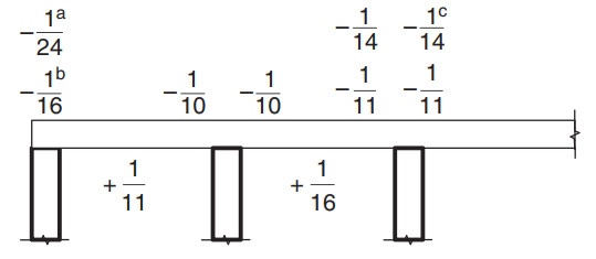
figura 8. Valori del coefficiente di momento \(\alpha\) per solai con più di due campate. (Yew-Chaye Loo & Sanual Abbraccio Chowdhury , “Cemento armato e precompresso”, 22a edizione, Cambridge University Press).
Dove:
- (un carico) Caso di solai e travi su travi portanti
- (b) Solo per supporto a trave continua
- (c) Dove viene utilizzato il rinforzo di classe L
- \(L_n \) è l'estensione unitaria della striscia
- \(F_d \) è il carico gravitazionale fattorizzato
Per l'esempio della lastra, dobbiamo usare il caso (un carico) perché la soletta poggia su travi rigide. Verrà spiegato solo un caso e il resto verrà mostrato nella tabella seguente. Includiamo anche il calcolo dell'area dell'armatura in acciaio.
- \(M={\alfa} {F_d}{L_n^2}={-\frac{1}{24}}\volte {13.89 \frac{kN}{m}}\volte (6m-0.5m)^2 = – 17.51{kN}{m}\)
- Copertura = 20mm (È necessario un minimo di 10 mm per un periodo di resistenza al fuoco di 60 minuti).
- \(d = t_{lastra} – Coperchio – \frac{Diametro barra}{2} = 250 mm – 20mm – 6millimetro = 224 mm \)
- \(\alfa_2 = 1.0-0.003 f’c = 1.0-0.003\times 25 = 0.925 (0.67 \le \alpha_2 \le 0.85) \) così, selezioniamo \(\alfa_2 = 0.85\)
- \(\xi = \frac{\alpha_2\times f’c}{f_{il suo}} = frac{0.85\volte 25 MPa}{500 MPa} = 0.0425 \)
- \(\rho_t = \xi – \sqrt{{\xi}^ 2 – \frac{{2}{\xi}{M}}{{\phi}{b}{d^2}{f_{il suo}}}} = 0.0425 – \sqrt{{0.0425}^2-\frac{2\times 0.0425\times 17.51{kN}{m}}{{0.8}\volte {1m}\volte {{(0.224m)^ 2}} \volte {500\volte {10^ 3}kPa}}}=0.0008814\)
- \(\gamma= 1.05-0.007 f’c = 1.05-0.007\times 25 = 0.875 (0.67 \le \gamma \le 0.85) \) così, selezioniamo \(\gamma = 0.85\)
- \(k_u = \frac{\rho_t \times f_{il suo}}{0.85\times \gamma \times f’c}= Frac{0.0008814\volte 500 MPa}{0.85\volte 0.85 \volte 25 MPa} =0.0244\)
- \(\fi = 1.19 – \frac{13\Eurocodice di design con piastra di base in acciaio{u0}}{12} = 1.19 – \frac{13\volte 0.0244}{12} = 1.164 (0.6 \le \phi \le 0.8) \) così, selezioniamo \(\fi = 0.8\). Ok!.
- \(\rho_{t,min} = 0.20 {(\frac{D}{d})^ 2}{(\frac{f’_{ct,f}}{f_{il suo}})} = 0.20 \volte (\frac{0.25m}{0.224m})^2 \times \frac{0.6\volte sqrt{25MPa}}{500 MPa} = 0.0015\)
- \(UN_{sto}= massimo(\rho_{t,min}, \rho_t)\times b \times d = max(0.0015,0.0008814)\volte 1000 mm \times 224 millimetro = 334.82 mm^2 \)
| \(\alpha\) e Momenti | Esterno negativo sinistro | Esterno Positivo | Esterno negativo a destra | Interno sinistro negativo | Interno positivo | Interno negativo a destra |
|---|---|---|---|---|---|---|
| \(\alpha\) valore | -\(\frac{1}{24}\) | \(\frac{1}{11}\) | -\(\frac{1}{10}\) | \(\frac{1}{10}\) | \(\frac{1}{16}\) | \(\frac{1}{11}\) |
| Valore M | -17.51 | 38.20 | -42.02 | 42.02 | 26.26 | 38.20 |
| \(\rho_t\) | 0.0008814 | 0.001948 | 0.002148 | 0.002148 | 0.00133 | 0.001948 |
| A | 0.0244 | 0.0539 | 0.0594 | 0.0594 | 0.0368 | 0.05391 |
| \(\phi\) | 0.8 | 0.8 | 0.8 | 0.8 | 0.8 | 0.8 |
| \(UN_{sto} {mm^2}\) | 334.82 | 436.31 | 481.099 | 481.099 | 334.8214 | 436.3100 |
Dopo il calcolo dell'area dell'armatura in acciaio, è possibile definire i dettagli (il modo effettivo di posizionare l'armatura nella soletta). Come aiuto per la tua conoscenza, condividiamo la seguente immagine, che indica la posizione dell'armatura per i momenti positivi e negativi:
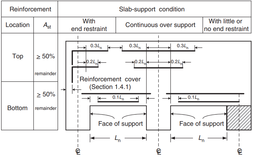
figura 9. Disposizione di armatura per lastre unidirezionali e bidirezionali. (Yew-Chaye Loo & Sanual Abbraccio Chowdhury , “Cemento armato e precompresso”, 22a edizione, Cambridge University Press)
Se sei nuovo in SkyCiv, Iscriviti e testa tu stesso il software!
Risultati del modulo di progettazione della piastra SkyCiv S3D
Nella prima vista, mostreremo alcune immagini per la modellazione e l'analisi strutturale dell'esempio in S3D. Ti consigliamo di leggere la modellazione in SkyCiv nei seguenti collegamenti Come modellare i piatti? screenshot-di-AISI-Coldform-9 Esempio di progettazione di lastre ACI con SkyCiv.
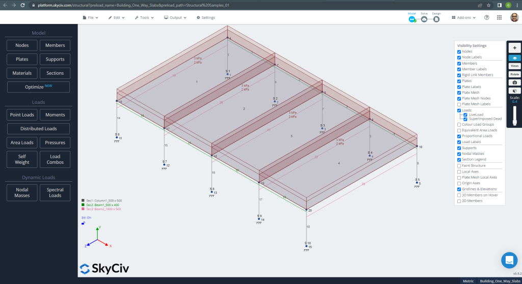
figura 10. Esempio di modello strutturale in S3D per solai unidirezionali. (3D strutturale, Ingegneria del cloud SkyCiv).
Prima di analizzare il modello, dobbiamo definire una dimensione della maglia della piastra. Alcuni riferimenti (2) consiglia una dimensione per l'elemento shell di 1/6 del breve arco o 1/8 del lungo arco, il più corto di loro. A seguito di questo valore, noi abbiamo \(\frac{L2}{6}= Frac{6m}{6} = 1 m \) o \(\frac{L1}{8}= Frac{14m}{8}= 1,75 m \); prendiamo 1 m come dimensione massima consigliata e 0,50 m di dimensione della maglia applicata.
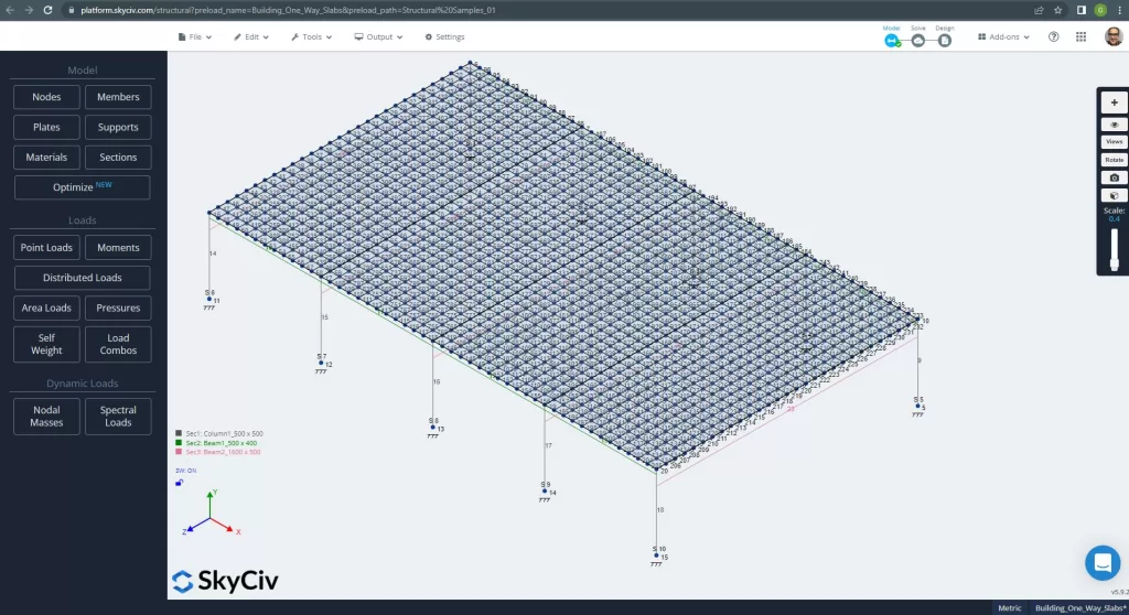
figura 11. Maglia migliorata nelle piastre. (3D strutturale, Ingegneria del cloud SkyCiv).
Una volta migliorato il nostro modello strutturale analitico, eseguiamo un'analisi elastica lineare. Quando si progettano lastre, dobbiamo verificare se gli spostamenti verticali sono inferiori al massimo consentito dal codice. Gli standard australiani hanno stabilito uno spostamento verticale massimo di manutenibilità di \(\frac{L}{250}= Frac{6000mm}{250}=24,0mm).
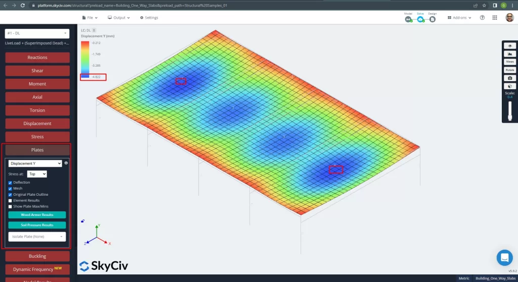
figura 12. Spostamento verticale nei piatti. (3D strutturale, Ingegneria del cloud SkyCiv).
Confronto tra lo spostamento verticale massimo e il valore di riferimento del codice, la rigidezza della soletta è adeguata. \(4.822 mm < 24.00mm\).
I momenti massimi nelle luci della soletta si trovano per positivo al centro e per negativo agli appoggi esterni ed interni. Vediamo i valori di questi momenti nelle seguenti immagini.
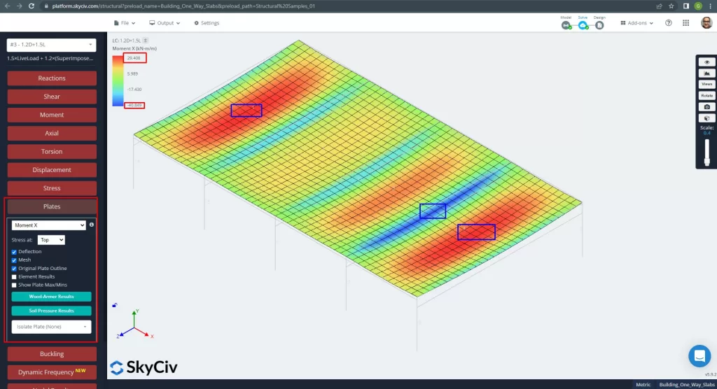
figura 13. Momenti nella direzione X. (3D strutturale, Ingegneria del cloud SkyCiv).
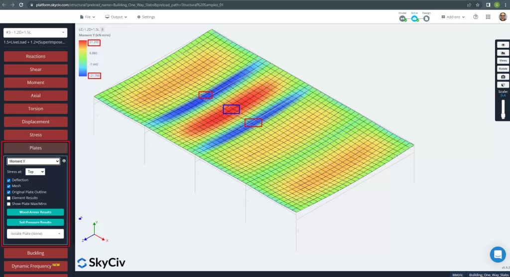
figura 14. Momenti nella direzione Y. (3D strutturale, Ingegneria del cloud SkyCiv).
Di seguito sono indicati gli assi locali dell'elemento piatto.
figura 15. Assi locali della soletta. (3D strutturale, Ingegneria del cloud SkyCiv).
Per maggiori dettagli sulla progettazione automatizzata di solette armate, vedere la nostra documentazione Targhe in SkyCiv.
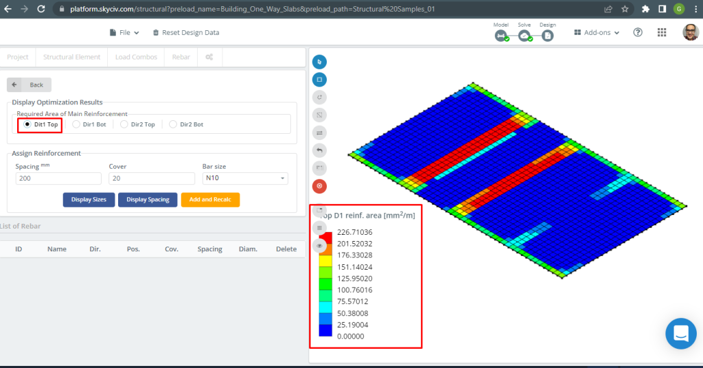
figura 16. Rinforzo superiore D1. (3D strutturale, Ingegneria del cloud SkyCiv).
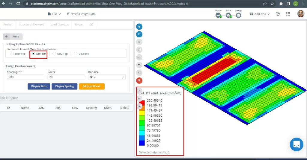
figura 17. Rinforzo inferiore D1. (3D strutturale, Ingegneria del cloud SkyCiv).
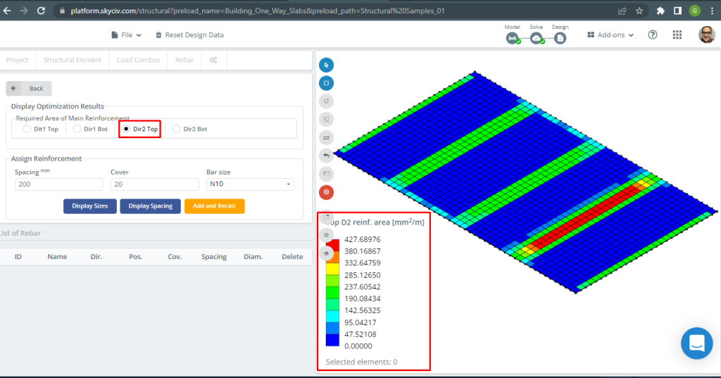
figura 18. Rinforzo superiore D2. (3D strutturale, Ingegneria del cloud SkyCiv).
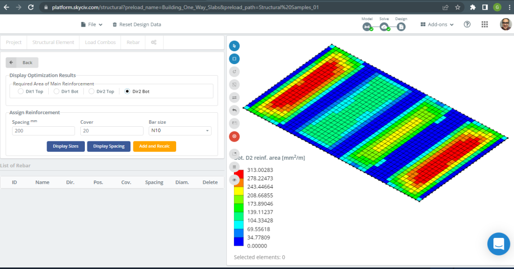
figura 19. Rinforzo inferiore D2. (3D strutturale, Ingegneria del cloud SkyCiv).
Confronto dei risultati
L'ultimo passaggio in questo esempio di progettazione di solaio unidirezionale è confrontare l'area dell'armatura in acciaio ottenuta dall'analisi S3D (assi locali “2”) e calcoli manuali.
| Momenti e area d'acciaio | Esterno negativo sinistro | Esterno Positivo | Esterno negativo a destra | Interno sinistro negativo | Interno positivo | Interno negativo a destra |
|---|---|---|---|---|---|---|
| \(UN_{sto, HandCalc} {mm^2}\) | 334.82 | 436.31 | 481.099 | 481.099 | 334.8214 | 436.3100 |
| \(UN_{sto, S3D} {mm^2}\) | 285.13 | 313.00 | 427.69 | 427.69 | 313.00 | 427.69 |
| \(\Delta_{dif}\) (%) | 14.84 | 28.262 | 11.101 | 11.101 | 6.517 | 1.986 |
Possiamo vedere che i risultati dei valori sono molto vicini tra loro. Questo significa che i calcoli sono corretti!
Esempio di progettazione di solette a due vie
In questa sezione, svilupperemo un esempio che consiste in un sistema di grillage.
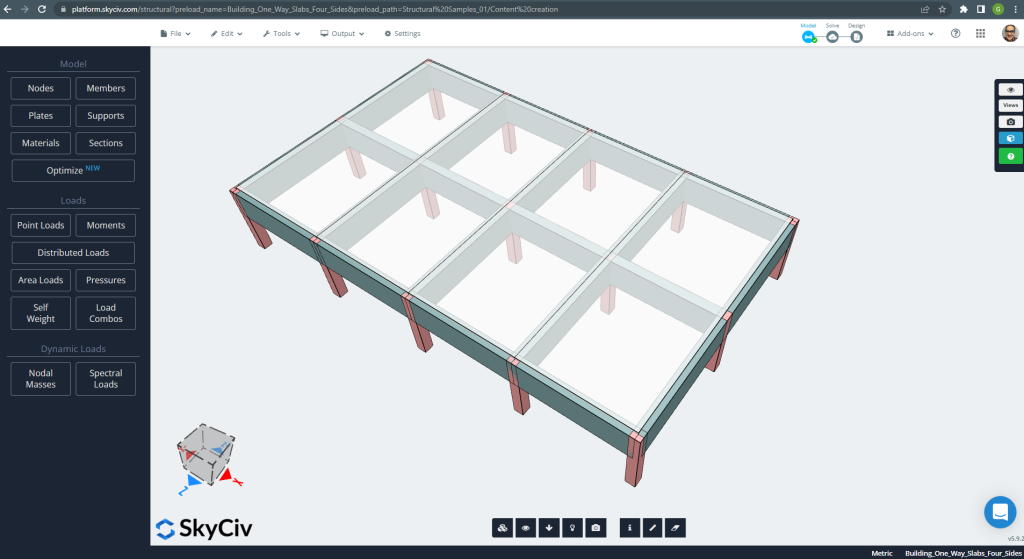
figura 20. Sistema di grigliatura. (3D strutturale, Ingegneria del cloud SkyCiv).
Le dimensioni del piano sono riportate di seguito
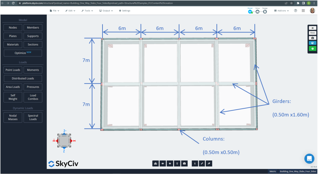
figura 21. Dimensioni in pianta per l'esempio di solaio bidirezionale sui quattro lati. (3D strutturale, Ingegneria del cloud SkyCiv).
Per l'esempio della lastra, In sintesi, il materiale, proprietà degli elementi, e carichi da considerare :
- Classificazione del tipo di soletta: Due – modo di comportamento \(\frac{L_2}{L_1} \il 2 ; \frac{7m}{6m}=1.167 < 2.00 \) Ok!
- Occupazione edilizia: Uso residenziale
- Spessore lastra \(t_{lastra}=0,25 m)
- Densità del cemento armato assumendo un rapporto di armatura in acciaio di 0.5% \(\ro_w = 24 \frac{kN}{m^3} + 0.6 \frac{kN}{m^3} \volte 0.5 = 24.3 \frac{kN}{m^3} \)
- Resistenza a compressione caratteristica del calcestruzzo a 28 giorni \(f'c = 25 MPa \)
- Modulo di elasticità del calcestruzzo secondo lo standard australiano \(E_c = 26700 MPa \)
- Peso proprio della lastra \(Dead = \rho_w \times t_{lastra} = 24.3 \frac{kN}{m^3} \volte 0,25 m = 6.075 \frac {kN}{m^2}\)
- Carico morto sovrapposto \(SD = 3.0 \frac {kN}{m^2}\)
- Carica in tempo reale \(L = 2.0 \frac {kN}{m^2}\)
Calcolo manuale secondo lo standard AS3600
In questa sezione, calcoleremo l'armatura in acciaio rinforzato richiesta utilizzando il riferimento dello standard australiano. Si ottiene dapprima il momento flettente totale fattorizzato che deve essere svolto dalle strisce di larghezza unitaria della soletta in ciascuna direzione principale di flessione.
- Carico morto, \(g = (3.0 + 6.075) \frac{kN}{m^2} \volte 1 m = 9.075 \frac{kN}{m}\)
- Carica in tempo reale, \(q = (2.0) \frac{kN}{m^2} \volte 1 m = 2.0 \frac{kN}{m}\)
- Carico finale, \(Fd = 1.2\times g + 1.5\volte q = (1.2\volte 9.075 + 1.5\volte 2.0)\frac{kN}{m} =13.89 \frac{kN}{m} \)
Momenti e coefficienti di progetto
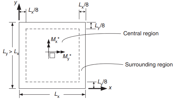
figura 22. Orientamento di una soletta bidirezionale per la determinazione dei momenti positivi. (Yew-Chaye Loo & Sanual Abbraccio Chowdhury , “Cemento armato e precompresso”, 22a edizione, Cambridge University Press)
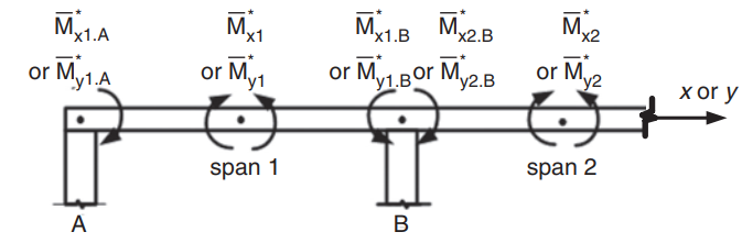
figura 23. Determinazione dei momenti negativi in una soletta bidirezionale. (Yew-Chaye Loo & Sanual Abbraccio Chowdhury , “Cemento armato e precompresso”, 22a edizione, Cambridge University Press)
| Condizione del bordo | Coefficienti di breve span (\(\beta_x\)) | Coefficienti a lungo raggio (\(\beta_y)\) tutti i valori di \(\frac{L_y}{L_x}\) | |||||||
|---|---|---|---|---|---|---|---|---|---|
| Valori di \(\frac{L_y}{L_x}\) | |||||||||
| 1.0 | 1.1 | 1.2 | 1.3 | 1.4 | 1.5 | 1.75 | \(\Metà dell'altezza del muro dal fondo della base per il caso del 2.0\) | ||
| 1. Quattro spigoli continui | 0.024 | 0.028 | 0.032 | 0.035 | 0.037 | 0.040 | 0.044 | 0.048 | 0.024 |
| 2. Un bordo corto discontinuos | 0.028 | 0.032 | 0.036 | 0.038 | 0.041 | 0.043 | 0.047 | 0.050 | 0.028 |
| 3. Un bordo lungo discontinuo | 0.028 | 0.035 | 0.041 | 0.046 | 0.050 | 0.054 | 0.061 | 0.066 | 0.028 |
| 4. Due bordi corti discontinui | 0.034 | 0.038 | 0.040 | 0.043 | 0.045 | 0.047 | 0.050 | 0.053 | 0.034 |
| 5. Due lembi lunghi discontinui | 0.034 | 0.046 | 0.056 | 0.065 | 0.072 | 0.078 | 0.091 | 0.100 | 0.034 |
| 6. Due spigoli adiacenti discontinui | 0.035 | 0.041 | 0.046 | 0.051 | 0.055 | 0.058 | 0.065 | 0.070 | 0.035 |
| 7. Tre spigoli discontinui (un bordo lungo continuo) | 0.043 | 0.049 | 0.053 | 0.057 | 0.061 | 0.064 | 0.069 | 0.074 | 0.043 |
| 8. Tre spigoli discontinui (un bordo corto continuo) | 0.043 | 0.054 | 0.064 | 0.072 | 0.078 | 0.084 | 0.096 | 0.105 | 0.043 |
| 9. Quattro spigoli discontinui | 0.056 | 0.066 | 0.074 | 0.081 | 0.087 | 0.093 | 0.103 | 0.111 | 0.056 |
tavolo 1. (Yew-Chaye Loo & Sanual Abbraccio Chowdhury , “Cemento armato e precompresso”, 22a edizione, Cambridge University Press)
L'immagine seguente spiega tutti e nove i casi a cui si riferisce la tabella sopra
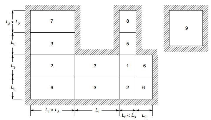
figura 24. Condizioni del bordo per lastre bidirezionali appoggiate su quattro lati. (Yew-Chaye Loo & Sanual Abbraccio Chowdhury , “Cemento armato e precompresso”, 22a edizione, Cambridge University Press)
Momenti di progettazione per la regione centrale (Astuccio 6 Due bordi adiacenti discontinui) :
- \(L_x = 6 m, L_y=7m, \frac{L_y}{L_x} = frac{7m}{6m}= 1.167 \) Valori da interpolare linearmente
- Positivi:
- \(M_x = {\beta_x}{F_d}{L_x^2} = {0.04435}\volte {13.89 \frac{kN}{m}}\volte{(6m)^ 2}=22.177 kNm\)
- \(M_a = {\beta_y}{F_d}{L_x^2} ={0.035}\volte {13.89 \frac{kN}{m}}\volte{(6m)^ 2}=17,501 kNm \)
- Negativi portata esterna:
- \(M_{x1,A} = -\lambda_e \times M_x = -0.5 \volte 22.177 kNm = – 11.089 kNm\)
- \(M_{y1,A} = -\lambda_e \times M_y = -0.5 \volte 17.501 kNm = -8.751 kNm \)
- Negativi portata interna:
- \(M_{x1, B} = -\lambda_{1x} \volte M_x = -1.33 \volte 22.177 kNm = – 29.495 kNm\)
- \(M_{y1, B} = -\lambda_{1y} \volte M_y = -1.33 \volte 17.501 kNm = -23.276 kNm \)
Momenti di progettazione per la regione centrale (Astuccio 3 Un bordo lungo discontinuo) :
- \(L_x = 6 m, L_y=7m, \frac{L_y}{L_x} = frac{7m}{6m}= 1.167 \) Valori da interpolare linearmente
- Positivi:
- \(M_x = {\beta_x}{F_d}{L_x^2} = {0.03902}\volte {13.89 \frac{kN}{m}}\volte{(6m)^ 2}= 19.512 kNm\)
- \(M_a = {\beta_y}{F_d}{L_x^2} ={0.028}\volte {13.89 \frac{kN}{m}}\volte{(6m)^ 2}= 14.001 kNm \)
- Negativi portata interna:
- \(M_{x1, B} = -\lambda_{1x} \volte M_x = -1.33 \volte 19.512 kNm = – 25.951 kNm\)
- \(M_{y1, B} = -\lambda_{1y} \volte M_y = -1.33 \volte 14.001 kNm = – 18.621 kNm \)
- Negativi interno seconda campata:
- \(M_{x2,B} = -\lambda_{2x} \volte M_x = -1.33 \volte 19.512 kNm = – 25.951 kNm\)
- \(M_{y2,B} = -\lambda_{2y} \volte M_y = -1.33 \volte 14.001 kNm = – 18.621 kNm \)
Acciaio per armature per la direzione X
| \(\alpha\) e Momenti | Esterno negativo sinistro | Esterno Positivo | Esterno negativo a destra | Interno sinistro negativo | Interno positivo | Interno negativo a destra |
|---|---|---|---|---|---|---|
| Valore M | 11.089 | 22.177 | 29.495 | 25.951 | 19.512 | 25.951 |
| \(\rho_t\) | 0.00055614 | 0.00112 | 0.001496 | 0.001313 | 0.000984 | 0.001313 |
| A | 0.015395 | 0.0310 | 0.0414 | 0.0364 | 0.0272 | 0.0364 |
| \(\phi\) | 0.8 | 0.8 | 0.8 | 0.8 | 0.8 | 0.8 |
| \(UN_{sto} {mm^2}\) | 334.8214 | 334.8214 | 335.08233 | 334.821 | 334.8214 | 334.8214 |
Acciaio per armature per la direzione Y
| \(\alpha\) e Momenti | Esterno negativo sinistro | Esterno Positivo | Esterno negativo a destra | Interno sinistro negativo | Interno positivo | Interno negativo a destra |
|---|---|---|---|---|---|---|
| Valore M | 8.751 | 17.501 | 23.276 | 18.621 | 14.001 | 18.621 |
| \(\rho_t\) | 0.0004383 | 0.0008811 | 0.001176 | 0.0009381 | 0.000703 | 0.0009381 |
| A | 0.0121 | 0.0244 | 0.03256 | 0.02597 | 0.0195 | 0.02597 |
| \(\phi\) | 0.8 | 0.8 | 0.8 | 0.8 | 0.8 | 0.8 |
| \(UN_{sto} {mm^2}\) | 334.821 | 334.821 | 334.821 | 334.821 | 334.8214 | 334.821 |
Se sei nuovo in SkyCiv, Iscriviti e testa tu stesso il software!
Risultati del modulo di progettazione della piastra SkyCiv S3D
Dopo aver perfezionato il modello, è il momento di eseguire un'analisi elastica lineare.
Quando si progettano lastre, dobbiamo verificare se gli spostamenti verticali sono inferiori al massimo consentito dal codice. Gli standard australiani hanno stabilito uno spostamento verticale massimo di manutenibilità di \(\frac{L}{250}= Frac{6000mm}{250}=24,0mm).
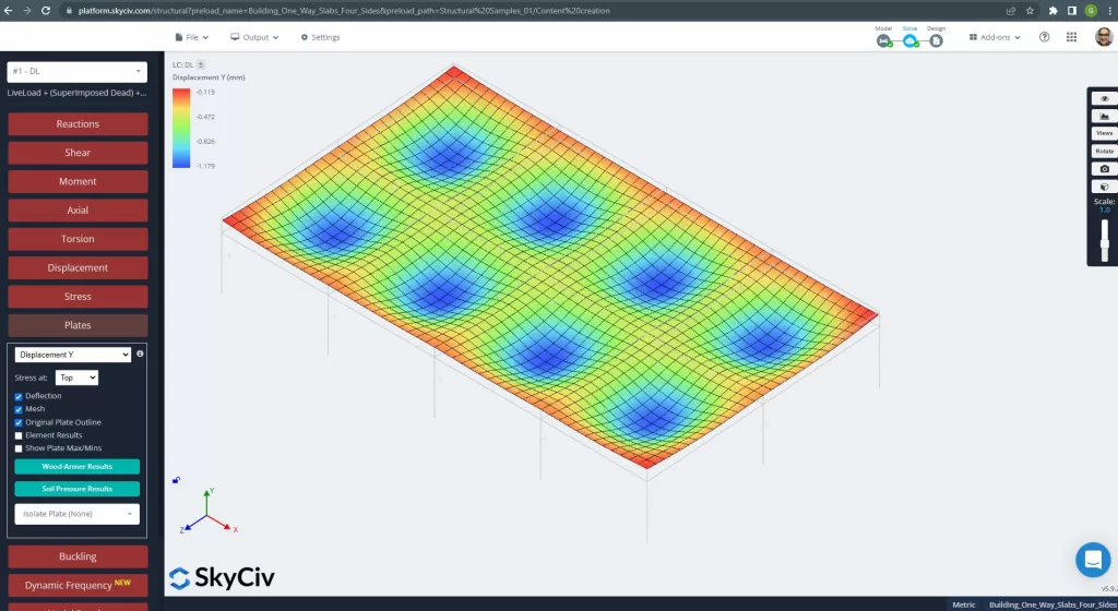
figura 25. Spostamento verticale nel sistema di piastre grillage. (3D strutturale, Ingegneria del cloud SkyCiv).
L'immagine sopra ci dà lo spostamento verticale. Il valore massimo è -1,179 mm, inferiore al massimo consentito di -24 mm. Pertanto, la rigidezza della soletta è adeguata.
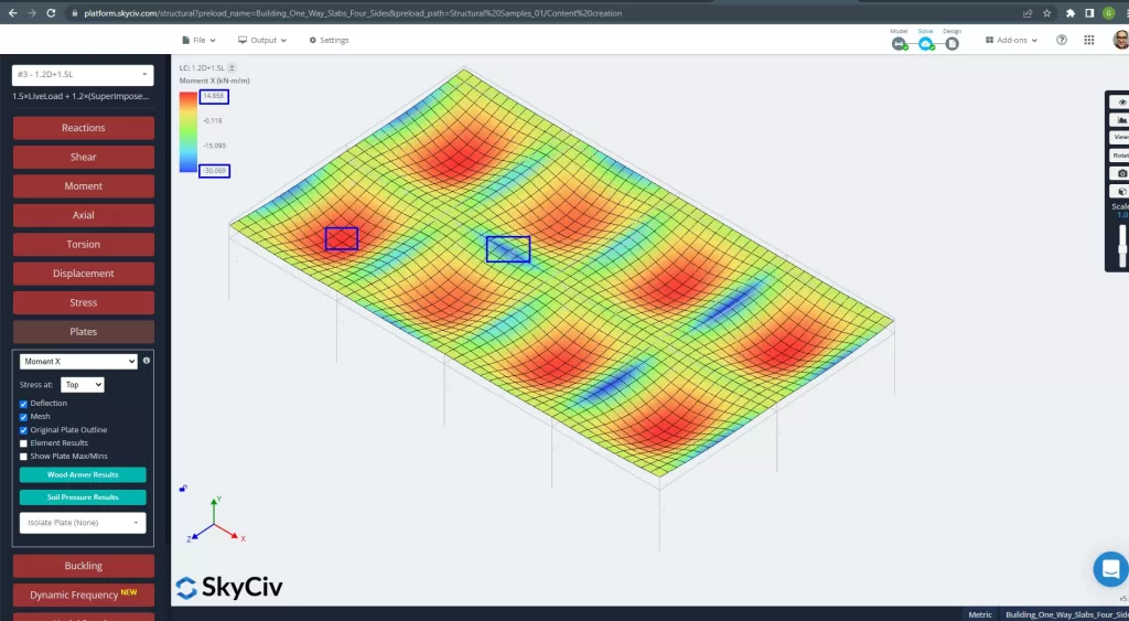
figura 26. Momenti delle piastre in direzione X. (3D strutturale, Ingegneria del cloud SkyCiv).
immagini 27 e 28 sono costituiti dal momento flettente in ciascuna direzione principale. Prendendo la distribuzione del momento ei valori, il software, SkyCiv, può quindi ottenere l'area totale dell'armatura in acciaio.
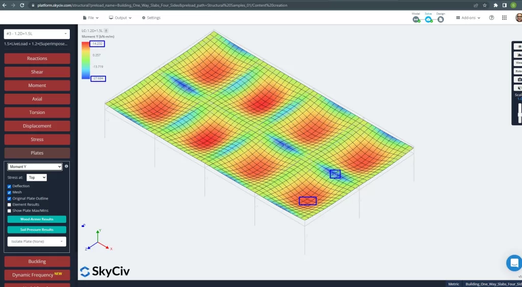
figura 27. Momenti delle piastre in direzione Y. (3D strutturale, Ingegneria del cloud SkyCiv).
Aree di rinforzo in acciaio:
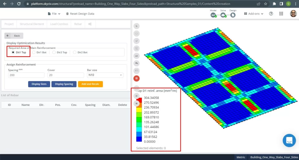
figura 28. Armatura in acciaio superiore in direzione 1. (3D strutturale, Ingegneria del cloud SkyCiv).
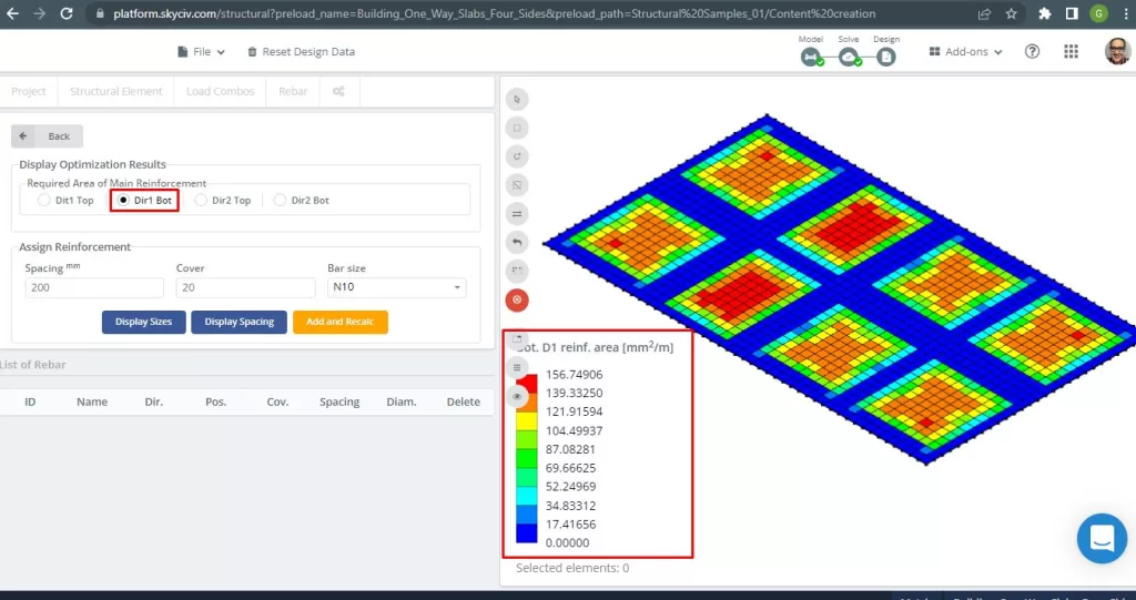
figura 29. Armatura inferiore dell'armatura in acciaio nella direzione 1. (3D strutturale, Ingegneria del cloud SkyCiv).
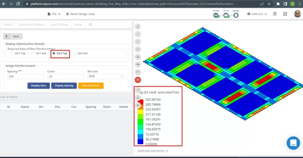
figura 30. Armatura in acciaio superiore in direzione 2. (3D strutturale, Ingegneria del cloud SkyCiv).
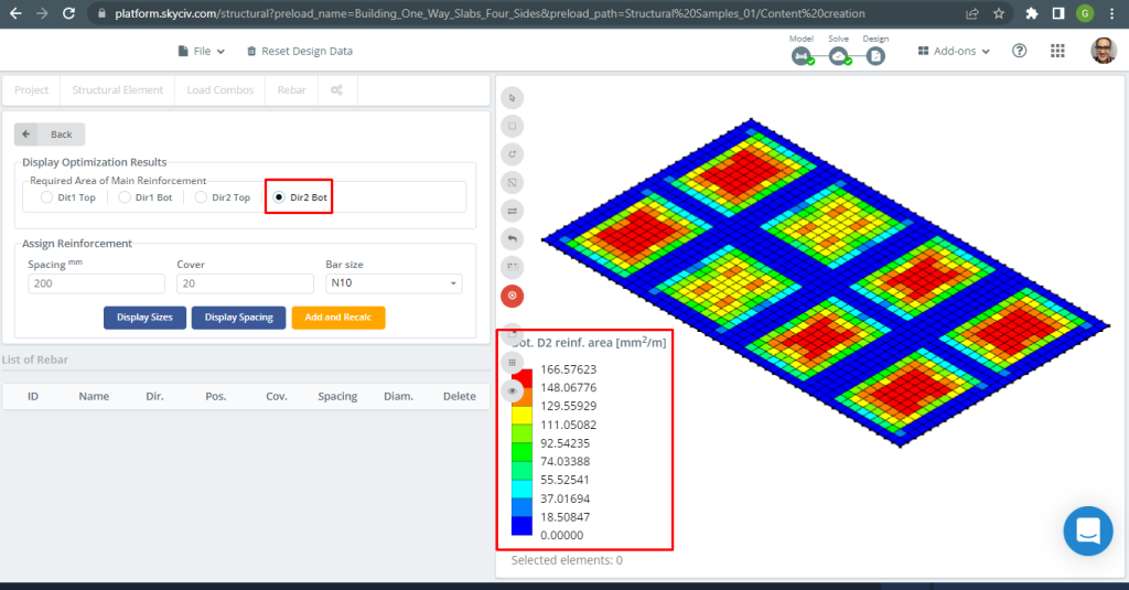
figura 31. Armatura inferiore dell'armatura in acciaio nella direzione 2. (3D strutturale, Ingegneria del cloud SkyCiv).
Confronto dei risultati
L'ultimo passaggio in questo esempio di progettazione di solai unidirezionali è il confronto dell'area dell'armatura in acciaio ottenuta dall'analisi S3D e dai calcoli manuali.
Acciaio per armature per la direzione X
| Momenti e area d'acciaio | Esterno negativo sinistro | Esterno Positivo | Esterno negativo a destra | Interno sinistro negativo | Interno positivo | Interno negativo a destra |
|---|---|---|---|---|---|---|
| \(UN_{sto, HandCalc} {mm^2}\) | 334.8214 | 334.8214 | 335.08233 | 334.821 | 334.8214 | 334.8214 |
| \(UN_{sto, S3D} {mm^2}\) | 289.75 | 149.35 | 325.967 | 325.967 | 116.16 | 217.311 |
| \(\Delta_{dif}\) (%) | 13.461 | 55.39 | 2.720 | 2.644 | 65.307 | 35.0964 |
Acciaio per armature per la direzione Y
| Momenti e area d'acciaio | Esterno negativo sinistro | Esterno Positivo | Esterno negativo a destra | Interno sinistro negativo | Interno positivo | Interno negativo a destra |
|---|---|---|---|---|---|---|
| \(UN_{sto, HandCalc} {mm^2}\) | 334.821 | 334.821 | 334.821 | 334.821 | 334.821 | 334.821 |
| \(UN_{sto, S3D} {mm^2}\) | 270.524 | 156.75 | 304.34 | 304.34 | 156.75 | 270.52 |
| \(\Delta_{dif}\) (%) | 19.203 | 53.184 | 9.104 | 9.104 | 53.184 | 19.204 |
La differenza è piuttosto elevata per i momenti positivi e la ragione sarebbe la presenza di travi con elevata rigidezza torsionale che influiscono sui risultati dell'analisi agli elementi finiti della piastra e sui calcoli per l'acciaio di armatura a flessione.
Se sei nuovo in SkyCiv, Iscriviti e testa tu stesso il software!
Riferimenti
- Yew-Chaye Loo & Sanual Abbraccio Chowdhury , “Cemento armato e precompresso”, 22a edizione, Cambridge University Press.
- Bazan Enrico & Melì Piralla, “Progettazione Sismica delle Strutture”, 1ed, CHIARO.
- Standard australiano, Strutture in cemento, AS 3600:2018