Systèmes de dalles considérés par la norme
Les normes australiennes établissent les exigences minimales pour la conception des dalles en béton armé, tels que les types unidirectionnels et bidirectionnels. Concernant la configuration du plan et l'inclusion des poutres, les dalles peuvent également être divisées en dalles soutenues sur quatre côtés, systèmes poutre-dalle, dalles plates, et assiettes plates. Ces types sont résumés dans les images suivantes.
Simplifiez la conformité de la conception des dalles australiennes avec les fonctionnalités avancées de SkyCiv exemple-de-rapport-concret. Essayez-le! Appliquez facilement AS 3600 contrôle les dalles et les plaques planes.
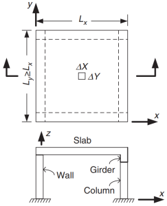
Figure 1. Dalle appuyée sur quatre côtés. (Yew-Chaye Loo & Sanual Hug Chowdhury , “Béton armé et précontraint”, 2ème édition, la presse de l'Universite de Cambridge).
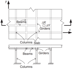
Figure 2. Système de dalle de grillage. (Yew-Chaye Loo & Sanual Hug Chowdhury , “Béton armé et précontraint”, 2ème édition, la presse de l'Universite de Cambridge).
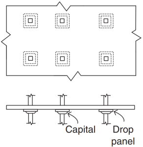
Figure 3. Dalles plates. (Yew-Chaye Loo & Sanual Hug Chowdhury , “Béton armé et précontraint”, 2ème édition, la presse de l'Universite de Cambridge).
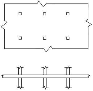
Figure 4. Assiettes Plates. (Yew-Chaye Loo & Sanual Hug Chowdhury , “Béton armé et précontraint”, 2ème édition, la presse de l'Universite de Cambridge).
La Norme recommande certaines méthodes (des procédures simplifiées et éprouvées) dans la détermination des moments de flexion:
- Clause 6.10.2: Poutres continues et dalles unidirectionnelles
- Clause 6.10.3: Dalles bidirectionnelles soutenues sur quatre côtés
- Clause 6.10.4: Dalles bidirectionnelles à portées multiples
Le but du code est de concevoir la quantité totale de barres d'armature en acier d'armature dans les directions principales du système de dalles. L'acier des barres d'armature sera calculé pour les moments de flexion “Mx” et “Mon.” Figure 5 montre les autres forces ou actions dans un élément de dalle fini dans lequel le code prescrit leurs valeurs de résistance.
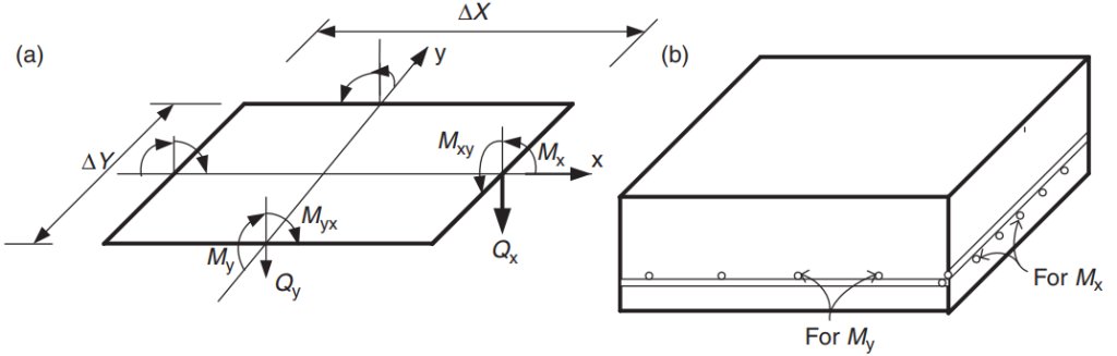
Figure 5. Forces dans un élément de dalle fini: moments de flexion (Mx, ma), moments bouleversants (Mxy, Myx), et des cisailles (Qx, Qy). (Yew-Chaye Loo & Sanual Hug Chowdhury , “Béton armé et précontraint”, 2ème édition, la presse de l'Universite de Cambridge)
Dans cet article, nous développerons deux exemples de conception de dalles, systèmes de dalles unidirectionnels et bidirectionnels, en utilisant les méthodes simplifiées orientées et permises par le code. Dans les deux cas, nous allons créer un modèle SkyCiv S3D et comparer les résultats avec les méthodes mentionnées ci-dessus.
Si vous êtes nouveau chez SkyCiv, Inscrivez-vous et testez le logiciel vous-même!
Exemple de conception de dalle unidirectionnelle
Ci-dessous, le petit bâtiment et les dalles que nous allons concevoir
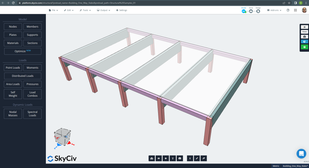
Figure 6. Exemple de dalles unidirectionnelles dans un petit bâtiment. (Structural 3D, Ingénierie Cloud SkyCiv).
Les dimensions du plan sont indiquées ci-dessous
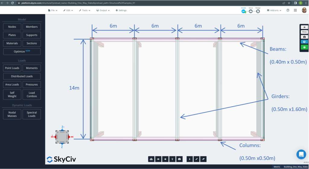
Figure 7. Dimensions du plan et éléments structurels. (Structural 3D, Ingénierie Cloud SkyCiv).
Pour l'exemple de la dalle, en résumé, le matériel, propriétés des éléments, et les charges à considérer :
- Classement des types de dalles: Une – comportement de manière \(\frac{L_2}{L_1} > 2 ; \frac{14m}{6m}=2,33 > 2.00 \) D'accord!
- Occupation du bâtiment: Usage résidentiel
- Épaisseur de la dalle \(t_{dalle}=0.25m\)
- Densité du béton armé en supposant un taux d'armature en acier de 0.5% \(\rho_w = 24 \frac{kN}{m^3} + 0.6 \frac{kN}{m^3} \fois 0.5 = 24.3 \frac{kN}{m^3} \)
- Résistance caractéristique à la compression du béton à 28 journées \(f'c = 25 MPa \)
- Module d'élasticité du béton selon la norme australienne \(E_c = 26700 MPa \)
- Poids propre de la dalle \(Dead = \rho_w \times t_{dalle} = 24.3 \frac{kN}{m^3} \fois 0.25m = 6.075 \frac {kN}{m^2}\)
- Charge morte superposée \(ET = 3.0 \frac {kN}{m^2}\)
- Charge vive \(L = 2.0 \frac {kN}{m^2}\)
Calcul manuel selon la norme AS3600
Dans cette section, nous calculerons les barres d'armature en acier renforcé requises en utilisant la référence de la norme australienne. Nous obtenons d'abord le moment de flexion total pondéré à effectuer par la bande de largeur unitaire de la dalle.
- Poids mort, \(g = (3.0 + 6.075) \frac{kN}{m^2} \fois 1 m = 9.075 \frac{kN}{m}\)
- Charge vive, \(q = (2.0) \frac{kN}{m^2} \fois 1 m = 2.0 \frac{kN}{m}\)
- Charge ultime, \(Fd = 1.2\times g + 1.5\fois q = (1.2\fois 9.075 + 1.5\fois 2.0)\frac{kN}{m} =13.89 \frac{kN}{m} \)
En utilisant la méthode simplifiée spécifiée par la norme, première, il est indispensable de respecter les restrictions suivantes:
- \(\frac{L_i}{L_j} \le 1.2 . \frac{6m}{6m} =1 < 1.2 \). D'accord!
- La charge doit être uniforme. D'accord!
- \(q \le 2g. q=2 \frac{kN}{m} < 18.15 \frac{kN}{m}\). D'accord!
- La section transversale de la dalle doit être uniforme. D'accord!.
Épaisseur minimale recommandée, d
\(d \ge \frac{L_{fe}}{{k_3}{k_4}{\sqrt[3]{\frac{\frac{\Delta}{L_{ef}}{E_c}}{F_{d, ef}}}}}\)
Où
- \(k_3 = 1.0; k_4 = 1.75 \)
- \(\frac{\Delta}{L_{ef}}=1/250 \)
- \(E_c = 27600 MPa \)
- \(F_{d,ef} = (1.0 +afin que les ingénieurs puissent revoir exactement comment ces calculs sont effectués{cs})\fois g + (\psi_s + afin que les ingénieurs puissent revoir exactement comment ces calculs sont effectués{cs}\times \psi_1) \fois q=(1.0+0.8)\fois 9.075 + (0.7+0.8\fois 0.4)\fois 2 = 18.375 kPa)
- \(\psi_s = 0.7 \) Facteur à court terme en charge vive
- \(\psi_1 = 0.4 \) Facteur de charge à long terme
- \(afin que les ingénieurs puissent revoir exactement comment ces calculs sont effectués{cs} = 0.8 \)
\(d \ge \frac{5.50m}{{1.0}\fois {1.75}{\sqrt[3]{\frac{\frac{1}{250}\fois{27600 \fois 10^3 kPa}}{18.375 kPa}}}} \ge 0,173m. d = 0,25 m > 0.173m \) D'accord!
Une fois que nous démontrons que les contraintes sont satisfaites, le moment de flexion est calculé à l'aide de l'expression: \(M=\alpha \times F_d \times L_n^2\) où \(\[object Window]) est une constante définie dans la figure suivante.
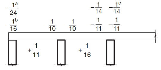
Figure 8. Valeurs du coefficient de moment \(\[object Window]) pour dalles à plus de deux travées. (Yew-Chaye Loo & Sanual Hug Chowdhury , “Béton armé et précontraint”, 2ème édition, la presse de l'Universite de Cambridge).
Où:
- (a) Cas des dalles et poutres sur support poutre
- (b) Pour support de poutre continue uniquement
- (c) Où un renfort de classe L est utilisé
- \(L_n \) est la portée unitaire de la bande
- \(F_d \) est la charge pondérée gravitationnelle
Pour l'exemple de la dalle, nous devons utiliser le cas (a) car la dalle repose sur des poutres rigides. Un seul cas sera expliqué et le reste sera présenté dans le tableau suivant. Nous incluons également le calcul de la surface d'armature en acier.
- \(M={\Il est important de mentionner que la distribution présentée et l'approche de calcul qui en résulte ne s'appliquent qu'aux pressions du sol agissant sur une face arrière verticale.} {F_d}{L_n^2}={-\frac{1}{24}}\fois {13.89 \frac{kN}{m}}\fois (6m-0.5m)À partir de l'élévation du sol générée à partir des élévations Google – 17.51{kN}{m}\)
- Couverture = 20 mm (Un minimum de 10 mm est nécessaire pour une période de résistance au feu de 60 minutes).
- \(d = t_{dalle} – Couverture – \frac{Diamètre de la barre}{2} = 250mm – 20mm – 6mm = 224 mm \)
- \(\alpha_2 = 1.0-0.003 f’c = 1.0-0.003\times 25 = 0.925 (0.67 \le \alpha_2 \le 0.85) \) C'est à dire, nous sélectionnons \(\alpha_2 = 0.85\)
- \(\xi = \frac{\alpha_2\times f’c}{F_{le sien}} = frac{0.85\fois 25 MPa}{500 MPa} = 0.0425 \)
- \(\rho_t = \xi – \sqrt{{\xi}^ 2 – \frac{{2}{\xi}{M}}{{\phi}{b}{j^2}{F_{le sien}}}} = 0.0425 – \sqrt{{0.0425}^2-\frac{2\times 0.0425\times 17.51{kN}{m}}{{0.8}\fois {1m}\fois {{(0.224m)^ 2}} \fois {500\fois {10^ 3}kPa}}}=0.0008814\)
- \(\gamma= 1.05-0.007 f’c = 1.05-0.007\times 25 = 0.875 (0.67 \le \gamma \le 0.85) \) C'est à dire, nous sélectionnons \(\gamma = 0.85\)
- \(k_u = \frac{\rho_t \times f_{le sien}}{0.85\times \gamma \times f’c}= frac{0.0008814\fois 500 MPa}{0.85\fois 0.85 \fois 25 MPa} =0.0244\)
- \(\phi = 1.19 – \frac{13\afin que les ingénieurs puissent revoir exactement comment ces calculs sont effectués{u0}}{12} = 1.19 – \frac{13\fois 0.0244}{12} = 1.164 (0.6 \le \phi \le 0.8) \) C'est à dire, nous sélectionnons \(\phi = 0.8\). D'accord!.
- \(\rho_{t,min} = 0.20 {(\frac{D}{d})^ 2}{(\frac{F'_{côté,F}}{F_{le sien}})} = 0.20 \fois (\frac{0.25m}{0.224m})^2 \times \frac{0.6\fois sqrt{25MPa}}{500 MPa} = 0.0015\)
- \(UNE_{st}=max(\rho_{t,min}, \rho_t)\times b \times d = max(0.0015,0.0008814)\fois 1000 mm \times 224 millimètre = 334.82 mm^2 \)
| \(\[object Window]) et instants | Extérieur négatif gauche | Extérieur positif | Extérieur négatif droit | Intérieur négatif gauche | Positif intérieur | Intérieur Négatif Droit |
|---|---|---|---|---|---|---|
| \(\[object Window]) value | -\(\frac{1}{24}\) | \(\frac{1}{11}\) | -\(\frac{1}{10}\) | \(\frac{1}{10}\) | \(\frac{1}{16}\) | \(\frac{1}{11}\) |
| Valeur M | -17.51 | 38.20 | -42.02 | 42.02 | 26.26 | 38.20 |
| \(\rho_t\) | 0.0008814 | 0.001948 | 0.002148 | 0.002148 | 0.00133 | 0.001948 |
| à | 0.0244 | 0.0539 | 0.0594 | 0.0594 | 0.0368 | 0.05391 |
| \(\phi\) | 0.8 | 0.8 | 0.8 | 0.8 | 0.8 | 0.8 |
| \(UNE_{st} {mm^2}\) | 334.82 | 436.31 | 481.099 | 481.099 | 334.8214 | 436.3100 |
Après le calcul de la surface des barres d'armature en acier, vous pouvez définir les détails (la manière réelle de placer le renfort dans la dalle). Comme aide pour votre connaissance, nous partageons l'image suivante, qui indique l'emplacement de l'armature pour les moments positifs et négatifs:
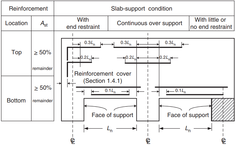
Figure 9. Armature de renfort pour dalles unidirectionnelles et bidirectionnelles. (Yew-Chaye Loo & Sanual Hug Chowdhury , “Béton armé et précontraint”, 2ème édition, la presse de l'Universite de Cambridge)
Si vous êtes nouveau chez SkyCiv, Inscrivez-vous et testez le logiciel vous-même!
Résultats du module de conception de plaques SkyCiv S3D
Dans la première vue, nous montrerons quelques images pour la modélisation et l'analyse structurelle de l'exemple en S3D. Nous vous recommandons de lire sur la modélisation dans SkyCiv dans les liens suivants Comment modéliser des plaques? Et Exemple de conception de dalle ACI avec SkyCiv.
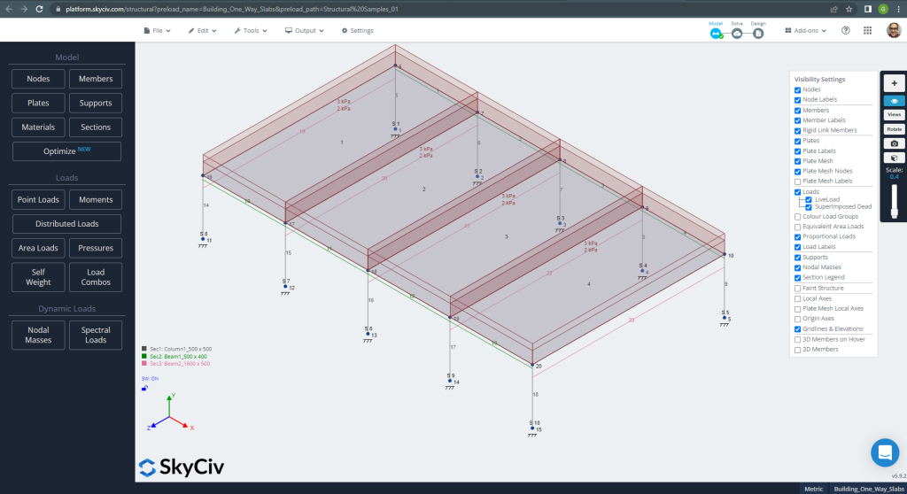
Figure 10. Modèle structurel en S3D pour exemple de dalles unidirectionnelles. (Structural 3D, Ingénierie Cloud SkyCiv).
Avant d'analyser le modèle, il faut définir un maillage de plaque. Quelques références (2) recommander une taille pour l'élément coque de 1/6 de la courte portée ou 1/8 de la longue portée, le plus court d'entre eux. Suite à cette valeur, nous avons \(\frac{L2}{6}= frac{6m}{6} = 1m \) ou \(\frac{L1}{8}= frac{14m}{8}=1.75m \); nous prenons 1 m comme taille maximale recommandée et 0,50 m de maillage appliqué.
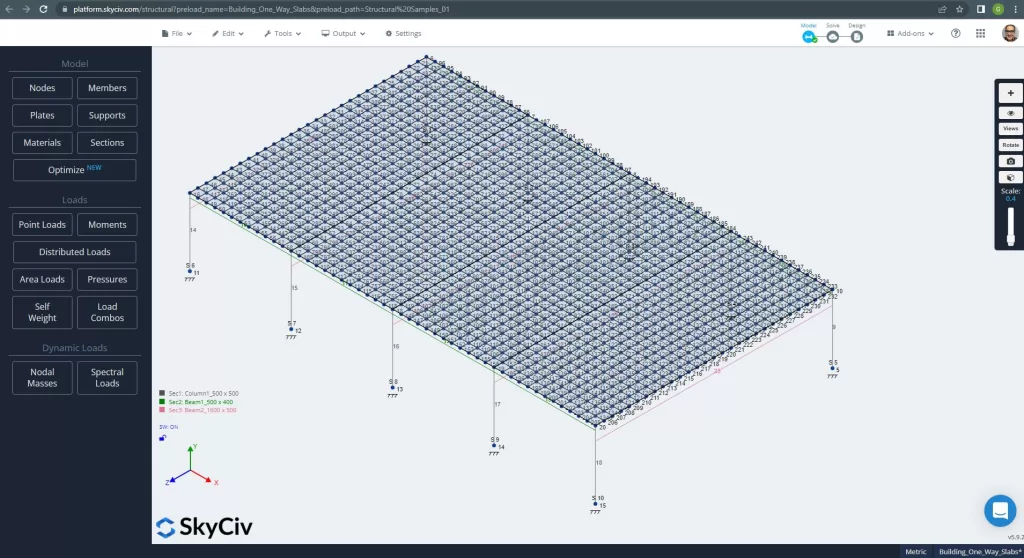
Figure 11. Maillage amélioré dans les plaques. (Structural 3D, Ingénierie Cloud SkyCiv).
Une fois que nous avons amélioré notre modèle structurel analytique, nous exécutons une analyse élastique linéaire. Lors de la conception des dalles, nous devons vérifier si le déplacement vertical est inférieur au maximum autorisé par le code. Les normes australiennes ont établi un déplacement vertical maximal de service de \(\frac{L}{250}= frac{6000mm}{250}=24.0 mm\).
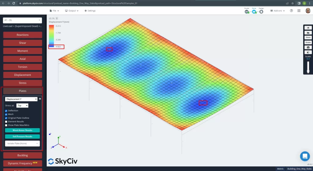
Figure 12. Déplacement vertical dans les plaques. (Structural 3D, Ingénierie Cloud SkyCiv).
Comparaison du déplacement vertical maximal avec la valeur référencée par le code, la rigidité de la dalle est suffisante. \(4.822 mm < 24.00mm).
Les moments maximaux dans les portées de la dalle sont situés pour le positif au centre et pour le négatif aux appuis extérieurs et intérieurs. Voyons ces valeurs de moments dans les images suivantes.
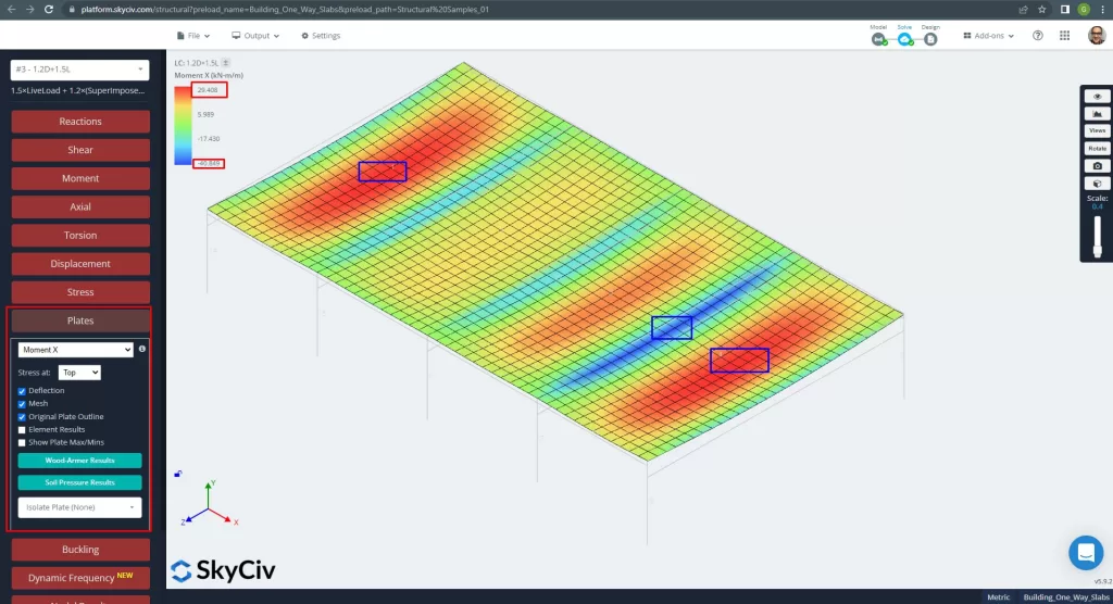
Figure 13. Moments dans la direction X. (Structural 3D, Ingénierie Cloud SkyCiv).
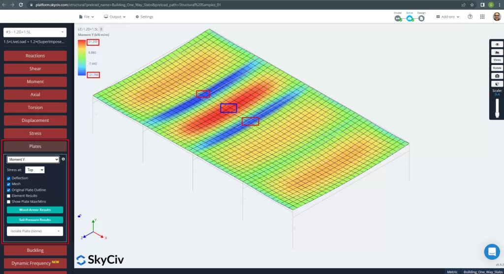
Figure 14. Moments dans la direction Y. (Structural 3D, Ingénierie Cloud SkyCiv).
Les axes locaux des éléments de plaque sont indiqués ci-dessous.
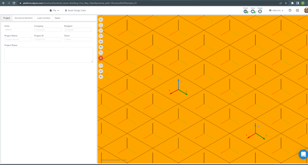
Figure 15. Axes locaux de la dalle. (Structural 3D, Ingénierie Cloud SkyCiv).
Pour plus de détails sur la conception automatisée des dalles renforcées, voir notre documentation Plaques dans SkyCiv.
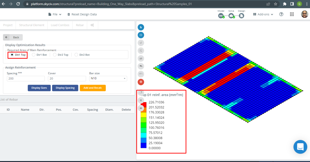
Figure 16. Renfort supérieur D1. (Structural 3D, Ingénierie Cloud SkyCiv).
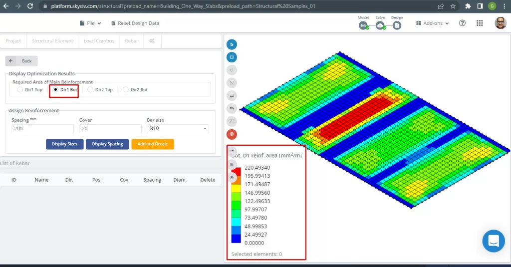
Figure 17. Renfort inférieur D1. (Structural 3D, Ingénierie Cloud SkyCiv).
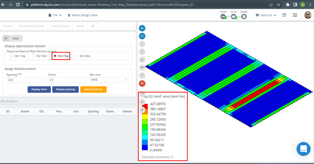
Figure 18. Renfort supérieur D2. (Structural 3D, Ingénierie Cloud SkyCiv).
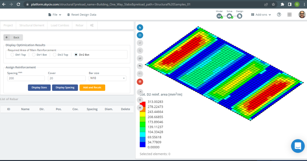
Figure 19. Renfort inférieur D2. (Structural 3D, Ingénierie Cloud SkyCiv).
Comparaison des résultats
La dernière étape de cet exemple de conception de dalle à sens unique consiste à comparer la zone d'armature en acier obtenue par analyse S3D (axes locaux “2”) et calculs manuels.
| Moments et zone d'acier | Extérieur négatif gauche | Extérieur positif | Extérieur négatif droit | Intérieur négatif gauche | Positif intérieur | Intérieur Négatif Droit |
|---|---|---|---|---|---|---|
| \(UNE_{st, Calculs manuels} {mm^2}\) | 334.82 | 436.31 | 481.099 | 481.099 | 334.8214 | 436.3100 |
| \(UNE_{st, S3D} {mm^2}\) | 285.13 | 313.00 | 427.69 | 427.69 | 313.00 | 427.69 |
| \(\Delta_{dif}\) (%) | 14.84 | 28.262 | 11.101 | 11.101 | 6.517 | 1.986 |
Nous pouvons voir que les résultats des valeurs sont très proches les uns des autres. Cela signifie que les calculs sont corrects!
Exemple de conception de dalle bidirectionnelle
Dans cette section, nous allons développer un exemple qui consiste en un système de grillage.
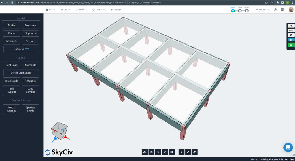
Figure 20. Système de grillage. (Structural 3D, Ingénierie Cloud SkyCiv).
Les dimensions du plan sont indiquées ci-dessous
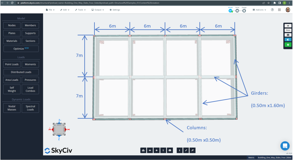
Figure 21. Dimensions en plan pour l'exemple de dalle à double sens sur les quatre côtés. (Structural 3D, Ingénierie Cloud SkyCiv).
Pour l'exemple de la dalle, en résumé, le matériel, propriétés des éléments, et les charges à considérer :
- Classement des types de dalles: Deux – comportement de manière \(\frac{L_2}{L_1} \le 2 ; \frac{7m}{6m}=1,167 < 2.00 \) D'accord!
- Occupation du bâtiment: Usage résidentiel
- Épaisseur de la dalle \(t_{dalle}=0.25m\)
- Densité du béton armé en supposant un taux d'armature en acier de 0.5% \(\rho_w = 24 \frac{kN}{m^3} + 0.6 \frac{kN}{m^3} \fois 0.5 = 24.3 \frac{kN}{m^3} \)
- Résistance caractéristique à la compression du béton à 28 journées \(f'c = 25 MPa \)
- Module d'élasticité du béton selon la norme australienne \(E_c = 26700 MPa \)
- Poids propre de la dalle \(Dead = \rho_w \times t_{dalle} = 24.3 \frac{kN}{m^3} \fois 0.25m = 6.075 \frac {kN}{m^2}\)
- Charge morte superposée \(ET = 3.0 \frac {kN}{m^2}\)
- Charge vive \(L = 2.0 \frac {kN}{m^2}\)
Calcul manuel selon la norme AS3600
Dans cette section, nous calculerons les barres d'armature en acier renforcé requises en utilisant la référence de la norme australienne. On obtient d’abord le moment de flexion total pondéré à réaliser par les bandes de largeur unitaire de la dalle dans chaque direction principale de flexion..
- Poids mort, \(g = (3.0 + 6.075) \frac{kN}{m^2} \fois 1 m = 9.075 \frac{kN}{m}\)
- Charge vive, \(q = (2.0) \frac{kN}{m^2} \fois 1 m = 2.0 \frac{kN}{m}\)
- Charge ultime, \(Fd = 1.2\times g + 1.5\fois q = (1.2\fois 9.075 + 1.5\fois 2.0)\frac{kN}{m} =13.89 \frac{kN}{m} \)
Moments de conception et coefficients
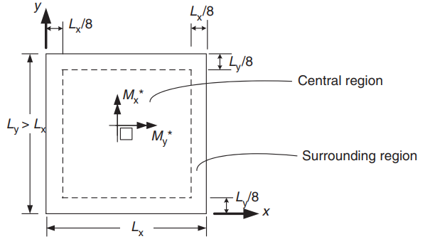
Figure 22. Orientation d'une dalle bidirectionnelle pour la détermination des moments positifs. (Yew-Chaye Loo & Sanual Hug Chowdhury , “Béton armé et précontraint”, 2ème édition, la presse de l'Universite de Cambridge)
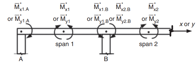
Figure 23. Détermination des moments négatifs dans une dalle bidirectionnelle. (Yew-Chaye Loo & Sanual Hug Chowdhury , “Béton armé et précontraint”, 2ème édition, la presse de l'Universite de Cambridge)
| État des bords | Coefficients de courte portée (\(\beta_x\)) | Coefficients de longue portée (\(\bêta_y)\) toutes les valeurs de \(\frac{L_y}{L_x}\) | |||||||
|---|---|---|---|---|---|---|---|---|---|
| Valeurs de \(\frac{L_y}{L_x}\) | |||||||||
| 1.0 | 1.1 | 1.2 | 1.3 | 1.4 | 1.5 | 1.75 | \(\cdot K_a 2.0\) | ||
| 1. Quatre bords continus | 0.024 | 0.028 | 0.032 | 0.035 | 0.037 | 0.040 | 0.044 | 0.048 | 0.024 |
| 2. Un bord court discontinu | 0.028 | 0.032 | 0.036 | 0.038 | 0.041 | 0.043 | 0.047 | 0.050 | 0.028 |
| 3. Un bord long discontinu | 0.028 | 0.035 | 0.041 | 0.046 | 0.050 | 0.054 | 0.061 | 0.066 | 0.028 |
| 4. Deux bords courts discontinus | 0.034 | 0.038 | 0.040 | 0.043 | 0.045 | 0.047 | 0.050 | 0.053 | 0.034 |
| 5. Deux longs bords discontinus | 0.034 | 0.046 | 0.056 | 0.065 | 0.072 | 0.078 | 0.091 | 0.100 | 0.034 |
| 6. Deux bords adjacents discontinus | 0.035 | 0.041 | 0.046 | 0.051 | 0.055 | 0.058 | 0.065 | 0.070 | 0.035 |
| 7. Trois bords discontinus (un bord long continu) | 0.043 | 0.049 | 0.053 | 0.057 | 0.061 | 0.064 | 0.069 | 0.074 | 0.043 |
| 8. Trois bords discontinus (un bord court continu) | 0.043 | 0.054 | 0.064 | 0.072 | 0.078 | 0.084 | 0.096 | 0.105 | 0.043 |
| 9. Quatre bords discontinus | 0.056 | 0.066 | 0.074 | 0.081 | 0.087 | 0.093 | 0.103 | 0.111 | 0.056 |
Le tableau 1. (Yew-Chaye Loo & Sanual Hug Chowdhury , “Béton armé et précontraint”, 2ème édition, la presse de l'Universite de Cambridge)
L'image suivante explique les neuf cas auxquels le tableau ci-dessus fait référence
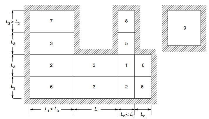
Figure 24. Conditions de bord pour les dalles bidirectionnelles appuyées sur quatre côtés. (Yew-Chaye Loo & Sanual Hug Chowdhury , “Béton armé et précontraint”, 2ème édition, la presse de l'Universite de Cambridge)
Moments de conception pour la région centrale (Cas 6 Deux bords adjacents discontinus) :
- \(L_x = 6m, L_y=7m, \frac{L_y}{L_x} = frac{7m}{6m}= 1.167 \) Valeurs à interpoler linéairement
- Points positifs:
- \(M_x = {\bêta_x}{F_d}{L_x^2} = {0.04435}\fois {13.89 \frac{kN}{m}}\fois{(6m)^ 2}=22.177 kNm\)
- \(M_y = {\bêta_y}{F_d}{L_x^2} ={0.035}\fois {13.89 \frac{kN}{m}}\fois{(6m)^ 2}=17.501kNm \)
- Portée extérieure négative:
- \(M_{x1,A} = -\lambda_e \times M_x = -0.5 \fois 22.177 kNm = – 11.089 kNm\)
- \(M_{y1,A} = -\lambda_e \times M_y = -0.5 \fois 17.501 kNm = -8.751 kNm \)
- Portée intérieure négative:
- \(M_{x1, B} = -\lambda_{1X} \fois M_x = -1.33 \fois 22.177 kNm = – 29.495 kNm\)
- \(M_{y1, B} = -\lambda_{1Y} \fois M_y = -1.33 \fois 17.501 kNm = -23.276 kNm \)
Moments de conception pour la région centrale (Cas 3 Un bord long discontinu) :
- \(L_x = 6m, L_y=7m, \frac{L_y}{L_x} = frac{7m}{6m}= 1.167 \) Valeurs à interpoler linéairement
- Points positifs:
- \(M_x = {\bêta_x}{F_d}{L_x^2} = {0.03902}\fois {13.89 \frac{kN}{m}}\fois{(6m)^ 2}= 19.512 kNm\)
- \(M_y = {\bêta_y}{F_d}{L_x^2} ={0.028}\fois {13.89 \frac{kN}{m}}\fois{(6m)^ 2}= 14.001 kNm \)
- Portée intérieure négative:
- \(M_{x1, B} = -\lambda_{1X} \fois M_x = -1.33 \fois 19.512 kNm = – 25.951 kNm\)
- \(M_{y1, B} = -\lambda_{1Y} \fois M_y = -1.33 \fois 14.001 kNm = – 18.621 kNm \)
- Négatifs intérieurs deuxième travée:
- \(M_{x2,B} = -\lambda_{2X} \fois M_x = -1.33 \fois 19.512 kNm = – 25.951 kNm\)
- \(M_{y2,B} = -\lambda_{2Y} \fois M_y = -1.33 \fois 14.001 kNm = – 18.621 kNm \)
Barres d'armature en acier pour la direction X
| \(\[object Window]) et instants | Extérieur négatif gauche | Extérieur positif | Extérieur négatif droit | Intérieur négatif gauche | Positif intérieur | Intérieur Négatif Droit |
|---|---|---|---|---|---|---|
| Valeur M | 11.089 | 22.177 | 29.495 | 25.951 | 19.512 | 25.951 |
| \(\rho_t\) | 0.00055614 | 0.00112 | 0.001496 | 0.001313 | 0.000984 | 0.001313 |
| à | 0.015395 | 0.0310 | 0.0414 | 0.0364 | 0.0272 | 0.0364 |
| \(\phi\) | 0.8 | 0.8 | 0.8 | 0.8 | 0.8 | 0.8 |
| \(UNE_{st} {mm^2}\) | 334.8214 | 334.8214 | 335.08233 | 334.821 | 334.8214 | 334.8214 |
Barres d'armature en acier pour la direction Y
| \(\[object Window]) et instants | Extérieur négatif gauche | Extérieur positif | Extérieur négatif droit | Intérieur négatif gauche | Positif intérieur | Intérieur Négatif Droit |
|---|---|---|---|---|---|---|
| Valeur M | 8.751 | 17.501 | 23.276 | 18.621 | 14.001 | 18.621 |
| \(\rho_t\) | 0.0004383 | 0.0008811 | 0.001176 | 0.0009381 | 0.000703 | 0.0009381 |
| à | 0.0121 | 0.0244 | 0.03256 | 0.02597 | 0.0195 | 0.02597 |
| \(\phi\) | 0.8 | 0.8 | 0.8 | 0.8 | 0.8 | 0.8 |
| \(UNE_{st} {mm^2}\) | 334.821 | 334.821 | 334.821 | 334.821 | 334.8214 | 334.821 |
Si vous êtes nouveau chez SkyCiv, Inscrivez-vous et testez le logiciel vous-même!
Résultats du module de conception de plaques SkyCiv S3D
Après avoir affiné le modèle, est-il temps d'exécuter une analyse élastique linéaire.
Lors de la conception des dalles, nous devons vérifier si le déplacement vertical est inférieur au maximum autorisé par le code. Les normes australiennes ont établi un déplacement vertical maximal de service de \(\frac{L}{250}= frac{6000mm}{250}=24.0 mm\).
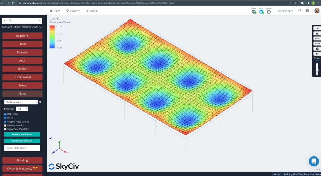
Figure 25. Déplacement vertical dans le système de dalles de grillage. (Structural 3D, Ingénierie Cloud SkyCiv).
L'image ci-dessus nous donne le déplacement vertical. La valeur maximale est de -1,179 mm, soit inférieure au maximum autorisé de -24 mm.. Par conséquent, la rigidité de la dalle est suffisante.
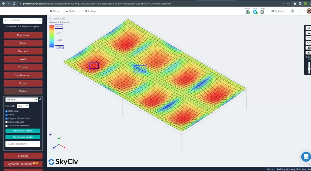
Figure 26. Moments des plaques dans la direction X. (Structural 3D, Ingénierie Cloud SkyCiv).
Images 27 et 28 se composent du moment de flexion dans chaque direction principale. Prendre la distribution et les valeurs du moment, les logiciels, SkyCiv, peut alors obtenir la surface totale d'armatures en acier.
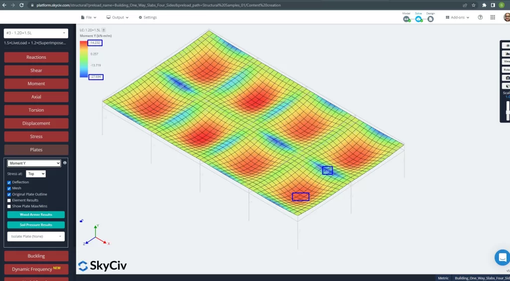
Figure 27. Moments des plaques dans la direction Y. (Structural 3D, Ingénierie Cloud SkyCiv).
Zones de renfort en acier:
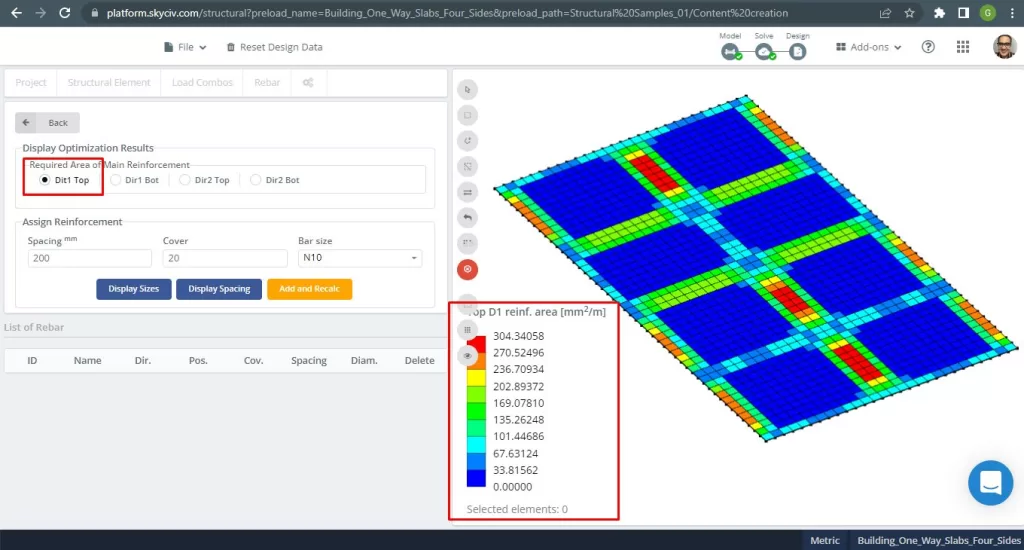
Figure 28. Renforcement supérieur des barres d'armature en acier dans la direction 1. (Structural 3D, Ingénierie Cloud SkyCiv).
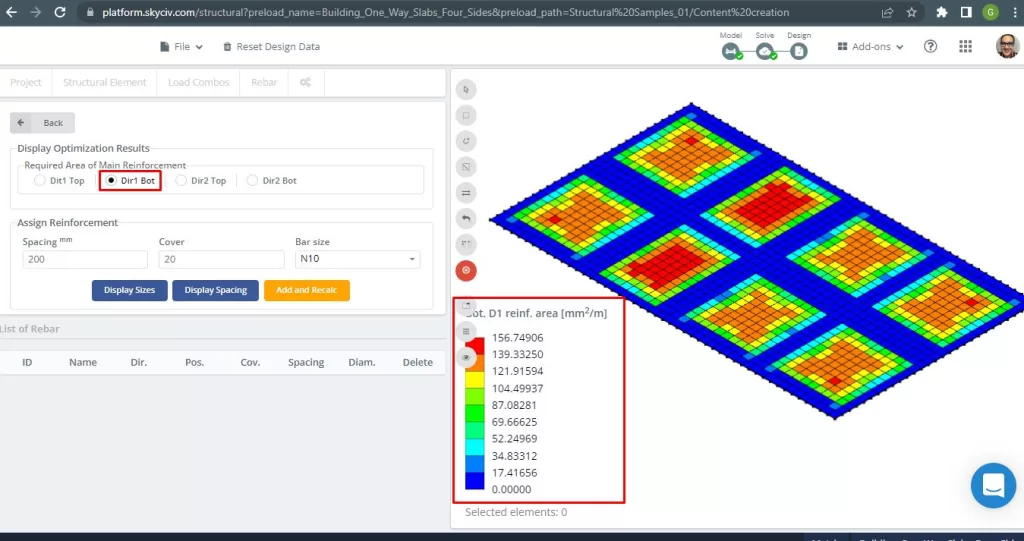
Figure 29. Renforcement des barres d'armature inférieures en acier dans la direction 1. (Structural 3D, Ingénierie Cloud SkyCiv).
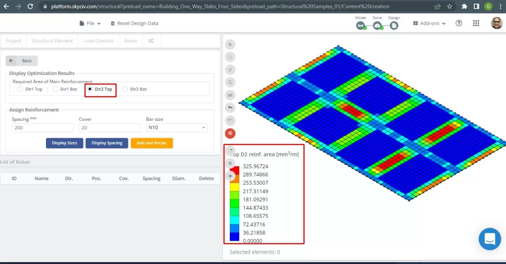
Figure 30. Renforcement supérieur des barres d'armature en acier dans la direction 2. (Structural 3D, Ingénierie Cloud SkyCiv).
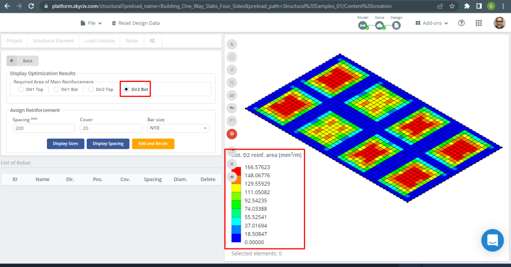
Figure 31. Renforcement des barres d'armature inférieures en acier dans la direction 2. (Structural 3D, Ingénierie Cloud SkyCiv).
Comparaison des résultats
La dernière étape de cet exemple de conception de dalle unidirectionnelle consiste à comparer la surface des barres d'armature en acier obtenue par analyse S3D et calculs manuels..
Barres d'armature en acier pour la direction X
| Moments et zone d'acier | Extérieur négatif gauche | Extérieur positif | Extérieur négatif droit | Intérieur négatif gauche | Positif intérieur | Intérieur Négatif Droit |
|---|---|---|---|---|---|---|
| \(UNE_{st, Calculs manuels} {mm^2}\) | 334.8214 | 334.8214 | 335.08233 | 334.821 | 334.8214 | 334.8214 |
| \(UNE_{st, S3D} {mm^2}\) | 289.75 | 149.35 | 325.967 | 325.967 | 116.16 | 217.311 |
| \(\Delta_{dif}\) (%) | 13.461 | 55.39 | 2.720 | 2.644 | 65.307 | 35.0964 |
Barres d'armature en acier pour la direction Y
| Moments et zone d'acier | Extérieur négatif gauche | Extérieur positif | Extérieur négatif droit | Intérieur négatif gauche | Positif intérieur | Intérieur Négatif Droit |
|---|---|---|---|---|---|---|
| \(UNE_{st, Calculs manuels} {mm^2}\) | 334.821 | 334.821 | 334.821 | 334.821 | 334.821 | 334.821 |
| \(UNE_{st, S3D} {mm^2}\) | 270.524 | 156.75 | 304.34 | 304.34 | 156.75 | 270.52 |
| \(\Delta_{dif}\) (%) | 19.203 | 53.184 | 9.104 | 9.104 | 53.184 | 19.204 |
La différence est assez élevée pour les moments positifs et la raison serait la présence de poutres avec une rigidité en torsion élevée qui a un impact sur les résultats de l'analyse par éléments finis des plaques et les calculs pour l'acier d'armature en flexion..
Si vous êtes nouveau chez SkyCiv, Inscrivez-vous et testez le logiciel vous-même!
Références
- Yew-Chaye Loo & Sanual Hug Chowdhury , “Béton armé et précontraint”, 2ème édition, la presse de l'Universite de Cambridge.
- Bazan Enrique & Méli Piralla, “Conception parasismique des structures”, 1ed, CLAIR.
- Norme australienne, Structures en Béton, AS 3600:2018