Exemple de conception de plaque de base en utilisant EN 1993-1-8:2005, EN 1993-1-1:2005, EN 1992-1-1:2004, et EN 1992-4:2018.
Déclaration de problème
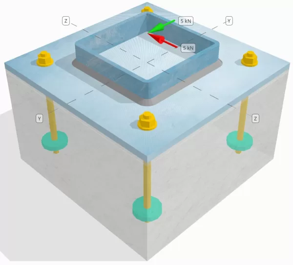
Déterminez si la connexion de colonne à base de colonne conçue est suffisante pour un Vy=5-kN et Vz=5-kN charges de cisaillement.
Données données
Colonne:
Section colonne: SHS180x180x8
Zone de colonne: 5440 mm2
Matériau de colonne: S235
Plaque de base:
Dimensions de la plaque de base: 350 millimètre x 350 mm
Épaisseur de plaque de base: 12 mm
Matériau de plaque de base: S235
Jointoyer:
Épaisseur de coulis: 6 mm
Matériau de coulis: ≥ 30 MPa
Béton:
Dimensions du béton: 350 millimètre x 350 mm
Épaisseur de béton: 350 mm
Matériau en béton: C25/30
Craquelé ou sans crates: Fissuré
Ancres:
Diamètre d'ancrage: 12 mm
Durée d'admission efficace: 150 mm
Diamètre de la plaque intégrée: 60 mm
Épaisseur de plaque intégrée: 10 mm
Matériau d'ancrage: 8.8
Autres informations:
- Ancrages non fraisés.
- Ancre à fils coupés.
- Facteur K7 pour la rupture par cisaillement de l'acier d'ancrage: 1.0
- Degré de retenue de la fixation: Aucune retenue
Soudures:
Type de soudure: Soudure d'angle
Taille de la jambe de soudure: 8mm
Classification du métal de remplissage: E35
Ancrer les données (de Calculateur de skyciv):
Modèle dans l'outil gratuit SkyCiv
Modélisez la conception de la plaque de base ci-dessus à l'aide de notre outil en ligne gratuit dès aujourd'hui.! Aucune inscription requise.
Définitions
Chemin de chargement:
Ce logiciel Logiciel de conception de plaque de base SkyCiv suit EN 1992-4:2018 pour conception de tige d'ancrage. Les charges de cisaillement appliquées au poteau sont transférées à la plaque de base via les soudures, puis au béton de support via les tiges d'ancrage.. Les pirènes de frottement et de cisaillement ne sont pas prises en compte dans cet exemple, Comme ces mécanismes ne sont pas pris en charge dans le logiciel actuel.
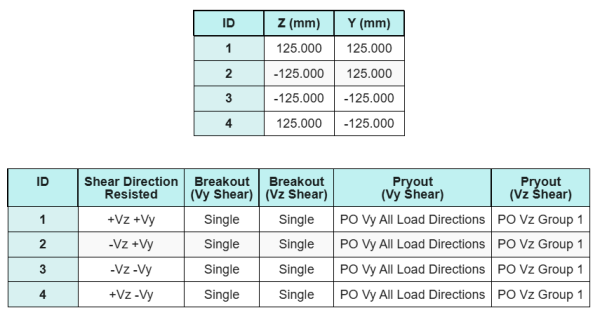
Groupes d'ancrage:
Le logiciel comprend une fonctionnalité intuitive qui identifie les ancres qui font partie d'un groupe d'ancres pour évaluer rupture de cisaillement en béton et cisaillement en béton échecs.
Un groupe d'ancrage est défini comme deux ancres ou plus avec des zones de résistance projetées qui se chevauchent. Dans le cas présent, Les ancres agissent ensemble, Et leur résistance combinée est vérifiée par rapport à la charge appliquée sur le groupe.
A ancre unique est défini comme une ancre dont la zone de résistance projetée ne chevauche aucune autre. Dans le cas présent, L'ancre agit seul, et la force de cisaillement appliquée sur cette ancre est vérifiée directement contre sa résistance individuelle.
Cette distinction permet au logiciel de capturer le comportement du groupe et les performances individuelles de l'ancrage lors de l'évaluation des modes de défaillance liés au cisaillement.
Calculs étape par étape
Vérifier #1: Calculer la capacité de soudure
Nous supposons que le Vz la charge de cisaillement est résistée par le soudures supérieure et inférieure, tandis que le Vy la charge de cisaillement est supportée exclusivement par le soudures gauche et droite.
Pour déterminer la capacité de soudure du soudures supérieure et inférieure, on calcule d'abord leur longueurs totales de soudure.
\(
L_{w,haut&bas} = 2 \la gauche(b_{col} – 2t_{col} – 2r_{col}\droite)
= 2 \fois gauche(180 \,\texte{mm} – 2 \fois 8 \,\texte{mm} – 2 \fois 4 \,\texte{mm}\droite)
= 312 \,\texte{mm}
\)
Prochain, on calcule le contraintes dans les soudures.
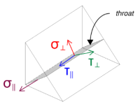
Notez que le cisaillement Vz appliqué agit parallèlement à l'axe de la soudure., sans aucune autre force présente. Cela signifie que les contraintes perpendiculaires peuvent être considérées comme nulles., et seulement le contrainte de cisaillement dans la direction parallèle il faut calculer.
\(
\sigma_{\perp} = frac{N}{(L_{w,haut&bas})\,asqrt{2}}
= frac{0 \,\texte{kN}}{(312 \,\texte{mm}) \fois 5.657 \,\texte{mm} \fois sqrt{2}}
= 0
\)
\(
\votre_{\perp} = frac{0}{(L_{w,haut&bas})\,asqrt{2}}
= frac{0 \,\texte{kN}}{(312 \,\texte{mm}) \fois 5.657 \,\texte{mm} \fois sqrt{2}}
= 0
\)
\(
\votre_{\parallèle} = frac{V_{z}}{(L_{w,haut&bas})\,a}
= frac{5 \,\texte{kN}}{(312 \,\texte{mm}) \fois 5.657 \,\texte{mm}}
= 2.8329 \,\texte{MPa}
\)
En utilisant EN 1993-1-8:2005, Eq. 4.1, la contrainte de soudure de conception est obtenue à l'aide de la méthode directionnelle.
\(
F_{w,Ed1} = sqrt{ (\sigma_{\perp})^ 2 + 3 \la gauche( (\votre_{\perp})^ 2 + (\votre_{\parallèle})^ 2 à droite) }
= sqrt{ (0)^ 2 + 3 \fois gauche( (0)^ 2 + (2.8329 \,\texte{MPa})^ 2 à droite) }
= 4.9067 \,\texte{MPa}
\)
Aussi, la contrainte normale de conception pour la vérification du métal de base, par EN 1993-1-8:2005, Eq. 4.1, est pris pour zéro, puisque pas de stress normal est présent.
\(
F_{w,Éd2} = sigma_{\perp} = 0
\)
Maintenant, évaluons le soudures gauche et droite. Comme pour les soudures supérieure et inférieure, on calcule d'abord le Longueur totale de soudure.
\(
L_{w,gauche&droite} = 2 \la gauche(ré_{col} – 2t_{col} – 2r_{col}\droite)
= 2 \fois gauche(180 \,\texte{mm} – 2 \fois 8 \,\texte{mm} – 2 \fois 4 \,\texte{mm}\droite)
= 312 \,\texte{mm}
\)
On calcule ensuite les composantes du contraintes de soudure.
\(
\sigma_{\perp} = frac{N}{(L_{w,gauche&droite})\,asqrt{2}}
= frac{0 \,\texte{kN}}{(312 \,\texte{mm}) \fois 5.657 \,\texte{mm} \fois sqrt{2}}
= 0
\)
\(
\votre_{\perp} = frac{0}{(L_{w,gauche&droite})\,asqrt{2}}
= frac{0 \,\texte{kN}}{(312 \,\texte{mm}) \fois 5.657 \,\texte{mm} \fois sqrt{2}}
= 0
\)
\(
\votre_{\parallèle} = frac{V_y}{(L_{w,gauche&droite})\,a}
= frac{5 \,\texte{kN}}{(312 \,\texte{mm}) \fois 5.657 \,\texte{mm}}
= 2.8329 \,\texte{MPa}
\)
En utilisant EN 1993-1-8:2005, Eq. 4.1, nous déterminons à la fois la contrainte de soudure de conception et la contrainte normale de conception pour le contrôle du métal de base.
\(
F_{w,Ed1} = sqrt{ \la gauche( \sigma_{\perp} \droite)^ 2 + 3 \la gauche( \la gauche( \votre_{\perp} \droite)^ 2 + \la gauche( \votre_{\parallèle} \droite)^ 2 à droite) }
\)
\(
F_{w,Ed1} = sqrt{ \la gauche( 0 \droite)^ 2 + 3 \fois gauche( \la gauche( 0 \droite)^ 2 + \la gauche( 2.8329 \,\texte{MPa} \droite)^ 2 à droite) }
\)
\(
F_{w,Ed1} = 4.9067 \,\texte{MPa}
\)
La prochaine étape consiste à identifier le régissant la contrainte de soudure entre les soudures haut/bas et les soudures gauche/droite. Parce que les longueurs de soudure sont égales et que les charges appliquées ont la même ampleur, les contraintes de soudure résultantes sont égales.
\(
F_{w,Ed1} = max(F_{w,Ed1}, \, F_{w,Ed1})
= max(4.9067 \,\texte{MPa}, \, 4.9067 \,\texte{MPa})
= 4.9067 \,\texte{MPa}
\)
La contrainte du métal de base reste nulle.
\(
F_{w,Éd2} = max(F_{w,Éd2}, \, F_{w,Éd2}) = max(0, \, 0) = 0
\)
Maintenant, nous calculons la capacité de soudure. Première, la résistance du soudure d'angle est calculé. ensuite, la résistance du métal commun est déterminé. Utiliser FR 1993-1-8:2005, Eq. 4.1, les capacités sont calculées comme suit:
\(
F_{w,Rd1} = frac{f_u}{\beta_w gauche(\gamma_{M2, soudure}\droite)}
= frac{360 \,\texte{MPa}}{0.8 \fois (1.25)}
= 360 \,\texte{MPa}
\)
\(
F_{w,Rd2} = frac{0.9 f_u}{\gamma_{M2, soudure}}
= frac{0.9 \fois 360 \,\texte{MPa}}{1.25}
= 259.2 \,\texte{MPa}
\)
Ensuite, nous comparons les contraintes de soudure avec les capacités de soudure, et les contraintes du métal de base avec les capacités du métal de base.
Puisque 4.9067 MPa < 360 MPa et 0 MPa < 259.2 MPa, la capacité de la connexion soudée est suffisant.
Vérifier #2: Calculer la capacité de rupture du béton en raison du cisaillement VY
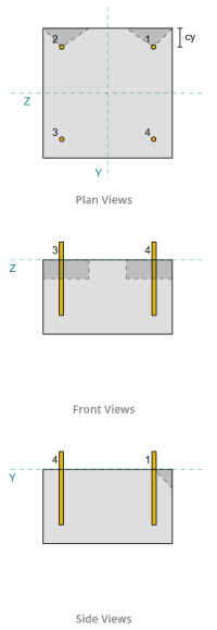
Suite aux dispositions de EN 1992-4:2018, le bord perpendiculaire à la charge appliquée est évalué pour la rupture par cisaillement. Seul le ancres les plus proches de ce bord sont considérés comme engagés, tandis que les ancrages restants sont supposés ne pas résister au cisaillement.
Ces ancrages de bord doivent avoir une distance au bord du béton supérieure à la plus grande de 10·hef et 60·d, où avoir est la longueur d'encastrement et d est le diamètre de l'ancre. Si cette condition n'est pas remplie, l'épaisseur de la plaque de base doit être inférieure à 0,25·hef.
Si les exigences de EN 1992-4:2018, Clause 7.2.2.5(1), ne sont pas satisfaits, le logiciel SkyCiv ne peut pas procéder aux vérifications de conception, et il est conseillé à l'utilisateur de se référer à d'autres normes pertinentes.
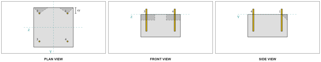
À partir des résultats du logiciel SkyCiv, les ancrages de bord agissent comme ancres simples, puisque leurs zones projetées ne se chevauchent pas. Pour ce calcul, Ancre 1 sera considéré.
Pour calculer la partie de la charge de cisaillement Vy supportée par Anchor 1, le cisaillement Vy total est réparti entre les ancrages les plus proches du bord. Cela donne le force perpendiculaire sur Ancre 1.
\(
V_{\perp} = frac{V_y}{n_{a,s}}
= frac{5 \,\texte{kN}}{2}
= 2.5 \,\texte{kN}
\)
Pour le force parallèle, on suppose que toutes les ancres résistent de la même manière à la charge. Par conséquent, la composante parallèle de la charge est calculée comme suit:
\(
V_{\parallèle} = frac{V_z}{n_{anc}}
= frac{5 \,\texte{kN}}{4}
= 1.25 \,\texte{kN}
\)
Ce logiciel Charge de cisaillement totale sur Ancre 1 est donc:
\(
V_{Ed} = sqrt{ \la gauche( V_{\perp} \droite)^ 2 + \la gauche( V_{\parallèle} \droite)^ 2 }
\)
\(
V_{Ed} = sqrt{ \la gauche( 2.5 \,\texte{kN} \droite)^ 2 + \la gauche( 1.25 \,\texte{kN} \droite)^ 2 } = 2.7951 \,\texte{kN}
\)
La première partie du calcul de capacité consiste à déterminer la facteurs alpha et bêta. Nous utilisons EN 1992-4:2018, Clause 7.2.2.5, pour régler le si dimension, et Équations 7.42 et 7.43 pour déterminer les facteurs.
\(
l_f = min(h_{ef}, \, 12ré_{anc})
= min(150 \,\texte{mm}, \, 12 \fois 12 \,\texte{mm})
= 144 \,\texte{mm}
\)
\(
\alpha = 0.1 \la gauche(\frac{l_f}{c_{1,s1}}\droite)^{0.5}
= 0.1 \fois gauche(\frac{144 \,\texte{mm}}{50 \,\texte{mm}}\droite)^{0.5}
= 0.16971
\)
\(
\bêta = 0.1 \la gauche(\frac{ré_{anc}}{c_{1,s1}}\droite)^{0.2}
= 0.1 \fois gauche(\frac{12 \,\texte{mm}}{50 \,\texte{mm}}\droite)^{0.2}
= 0.07517
\)
L'étape suivante consiste à calculer le valeur initiale de la résistance caractéristique de la fixation. En utilisant EN 1992-4:2018, Équation 7.41, la valeur est:
\(
V^{0}_{afin que les ingénieurs puissent revoir exactement comment ces calculs sont effectués,c} = k_9 gauche( \frac{ré_{anc}}{\texte{mm}} \droite)^{\Il est important de mentionner que la distribution présentée et l'approche de calcul qui en résulte ne s'appliquent qu'aux pressions du sol agissant sur une face arrière verticale.}
\la gauche( \frac{l_f}{\texte{mm}} \droite)^{\bêta}
\sqrt{ \frac{F_{afin que les ingénieurs puissent revoir exactement comment ces calculs sont effectués}}{\texte{MPa}} }
\la gauche( \frac{c_{1,s1}}{\texte{mm}} \droite)^{1.5} N
\)
\(
V^{0}_{afin que les ingénieurs puissent revoir exactement comment ces calculs sont effectués,c} = 1.7 \fois gauche( \frac{12 \,\texte{mm}}{1 \,\texte{mm}} \droite)^{0.16971}
\fois gauche( \frac{144 \,\texte{mm}}{1 \,\texte{mm}} \droite)^{0.07517}
\fois sqrt{ \frac{20 \,\texte{MPa}}{1 \,\texte{MPa}} }
\fois gauche( \frac{50 \,\texte{mm}}{1 \,\texte{mm}} \droite)^{1.5}
\fois 0.001 \,\texte{kN}
\)
\(
V^{0}_{afin que les ingénieurs puissent revoir exactement comment ces calculs sont effectués,c} = 5.954 \,\texte{kN}
\)
ensuite, Nous calculons le surface projetée de référence d'une seule ancre, Suivant EN 1992-4:2018, Équation 7.44.
\(
UNE_{c,V}^{0} = 4.5 \la gauche( c_{1,s1} \droite)^ 2
= 4.5 \fois gauche( 50 \,\texte{mm} \droite)^ 2
= 11250 \,\texte{mm}^ 2
\)
Après ça, Nous calculons le superficie réelle projetée d'Ancre 1.
\(
B_{c,V} = min(c_{la gauche,s1}, \, 1.5c_{1,s1}) + \min(c_{droite,s1}, \, 1.5c_{1,s1})
\)
\(
B_{c,V} = min(300 \,\texte{mm}, \, 1.5 \fois 50 \,\texte{mm}) + \min(50 \,\texte{mm}, \, 1.5 \fois 50 \,\texte{mm}) = 125 \,\texte{mm}
\)
\(
H_{c,V} = min(1.5c_{1,s1}, \, t_{concurrence}) = min(1.5 \fois 50 \,\texte{mm}, \, 200 \,\texte{mm}) = 75 \,\texte{mm}
\)
\(
UNE_{c,V} = H_{c,V} B_{c,V} = 75 \,\texte{mm} \fois 125 \,\texte{mm} = 9375 \,\texte{mm}^ 2
\)
Nous devons également calculer les paramètres de rupture en cisaillement. Nous utilisons EN 1992-4:2018, Équation 7.4, pour obtenir le facteur qui explique le perturbation de la répartition des contraintes, Équation 7.46 pour le facteur qui explique le épaisseur de la barre, et Équation 7.48 pour le facteur qui explique le influence d'une charge de cisaillement inclinée vers le bord. Ceux-ci sont calculés comme suit:
\(
\Psi_{s,V} = min gauche( 0.7 + 0.3 \la gauche( \frac{c_{2,s1}}{1.5c_{1,s1}} \droite), \, 1.0 \droite)
= min gauche( 0.7 + 0.3 \fois gauche( \frac{50 \,\texte{mm}}{1.5 \fois 50 \,\texte{mm}} \droite), \, 1 \droite)
= 0.9
\)
\(
\Psi_{h,V} = max gauche( \la gauche( \frac{1.5c_{1,s1}}{t_{concurrence}} \droite)^{0.5}, \, 1 \droite)
= max gauche( \la gauche( \frac{1.5 \fois 50 \,\texte{mm}}{200 \,\texte{mm}} \droite)^{0.5}, \, 1 \droite)
= 1
\)
\(
\alpha_{V} = tan^{-1} \la gauche( \frac{V_{\parallèle}}{V_{\perp}} \droite)
= tan^{-1} \la gauche( \frac{1.25 \,\texte{kN}}{2.5 \,\texte{kN}} \droite)
= 0.46365 \,\texte{travailler}
\)
\(
\Psi_{\Il est important de mentionner que la distribution présentée et l'approche de calcul qui en résulte ne s'appliquent qu'aux pressions du sol agissant sur une face arrière verticale.,V} = max gauche(
\sqrt{ \frac{1}{(\cos(\alpha_{V}))^ 2 + \la gauche( 0.5 \, (\sin(\alpha_{V})) \droite)^ 2 } }, \, 1 \droite)
\)
\(
\Psi_{\Il est important de mentionner que la distribution présentée et l'approche de calcul qui en résulte ne s'appliquent qu'aux pressions du sol agissant sur une face arrière verticale.,V} = max gauche(
\sqrt{ \frac{1}{(\cos(0.46365 \,\texte{travailler}))^ 2 + \la gauche( 0.5 \fois péché(0.46365 \,\texte{travailler}) \droite)^ 2 } }, \, 1 \droite)
\)
\(
\Psi_{\Il est important de mentionner que la distribution présentée et l'approche de calcul qui en résulte ne s'appliquent qu'aux pressions du sol agissant sur une face arrière verticale.,V} = 1.0847
\)
Une remarque importante lors de la détermination du facteur alpha est de s'assurer que le cisaillement perpendiculaire et le cisaillement parallèle sont correctement identifiés..
Ensuite, Nous calculons le résistance à l'évasion de l'ancre unique en utilisant EN 1992-4:2018, Équation 7.1.
\(
V_{afin que les ingénieurs puissent revoir exactement comment ces calculs sont effectués,c} =V^0_{afin que les ingénieurs puissent revoir exactement comment ces calculs sont effectués,c} \la gauche(\frac{UNE_{c,V}}{UNE^0_{c,V}}\droite)
\Psi_{s,V} \Psi_{h,V} \Psi_{ce,V} \Psi_{\Il est important de mentionner que la distribution présentée et l'approche de calcul qui en résulte ne s'appliquent qu'aux pressions du sol agissant sur une face arrière verticale.,V} \Psi_{= facteur de réduction pour filetage coupé,V}
\)
\(
V_{afin que les ingénieurs puissent revoir exactement comment ces calculs sont effectués,c} = 5.954 \,\texte{kN} \fois gauche(\frac{9375 \,\texte{mm}^ 2}{11250 \,\texte{mm}^ 2}\droite)
\fois 0.9 \fois 1 \fois 1 \fois 1.0847 \fois 1
= 4.8435 \,\texte{kN}
\)
Application du facteur partiel, la résistance de conception est 3.23 kN.
\(
V_{Rd,c} = frac{V_{afin que les ingénieurs puissent revoir exactement comment ces calculs sont effectués,c}}{\gamma_{Mc}}
= frac{4.8435 \,\texte{kN}}{1.5}
= 3.229 \,\texte{kN}
\)
Puisque 2.7951 kN < 3.229 kN, la capacité de rupture en cisaillement pour le cisaillement Vy est suffisant.
Vérifier #3: Calculer la capacité de rupture du béton dû au cisaillement VZ
La même approche est utilisée pour déterminer la capacité sur le bord perpendiculaire au cisaillement Vz.
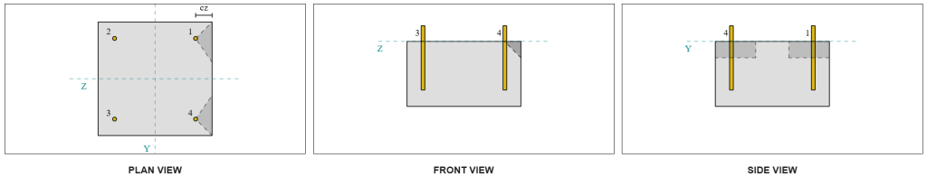
En raison de la conception symétrique, les ancrages résistant au cisaillement Vz sont également identifiés comme ancres simples. Voyons Ancre 1 encore une fois pour les calculs.
Pour calculer le charge perpendiculaire sur Ancre 1, nous divisons le cisaillement Vz par le nombre total d'ancrages les plus proches du bord uniquement. Pour calculer le charge parallèle sur Ancre 1, on divise le cisaillement Vy par le nombre total d'ancres.
\(
V_{\perp} = frac{V_{z}}{n_{a,s}}
= frac{5 \,\texte{kN}}{2}
= 2.5 \,\texte{kN}
\)
\(
V_{\parallèle} = frac{V_{Y}}{n_{anc}}
= frac{5 \,\texte{kN}}{4}
= 1.25 \,\texte{kN}
\)
\(
V_{Ed} = sqrt{ \la gauche( V_{\perp} \droite)^ 2 + \la gauche( V_{\parallèle} \droite)^ 2 }
\)
\(
V_{Ed} = sqrt{ \la gauche( 2.5 \,\texte{kN} \droite)^ 2 + \la gauche( 1.25 \,\texte{kN} \droite)^ 2 }
= 2.7951 \,\texte{kN}
\)
Utiliser une approche similaire pour Check #2, le résultat résistance à l'évasion car l’arête perpendiculaire au cisaillement Vz est:
\(
V_{Rd,c} = frac{V_{afin que les ingénieurs puissent revoir exactement comment ces calculs sont effectués,c}}{\gamma_{Mc}}
= frac{4.8435 \,\texte{kN}}{1.5}
= 3.229 \,\texte{kN}
\)
Puisque 2.7951 kN < 3.229 kN, la capacité de rupture en cisaillement pour le cisaillement Vz est suffisant.
Vérifier #4: Calculer la capacité de pryout en béton
Le calcul de la résistance au cisaillement consiste à déterminer le capacité nominale des ancrages contre la rupture par tension. La référence pour la capacité de rupture en tension est EN 1992-4:2018, Clause 7.2.1.4. Une discussion détaillée sur la rupture de tension est déjà couverte dans le Exemple de conception SkyCiv avec charge de tension et ne sera pas répété dans cet exemple de conception.
À partir des calculs du logiciel SkyCiv, la capacité nominale de la section pour la rupture en tension est 44.61 kN.
On utilise alors EN 1992-4:2018, Équation 7.39a, pour obtenir la résistance caractéristique de conception. En utilisant k8 = 2, la capacité est 59.48 kN.
\(
V_{Rd,cp} = frac{k_8 N_{cbg}}{\Gamma_c}
= frac{2 \fois 44.608 \,\texte{kN}}{1.5}
= 59.478 \,\texte{kN}
\)
Lors du contrôle de cisaillement, toutes les ancres sont efficaces en résistant à la pleine charge de cisaillement. À partir de l'image générée par le logiciel SkyCiv, toutes les projections du cône de rupture se chevauchent, faire en sorte que les ancres agissent comme un groupe d'ancrage.
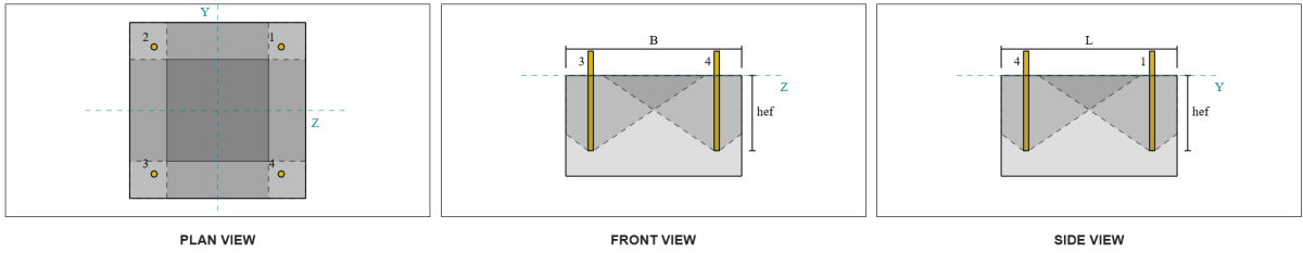
Par conséquent, la résistance requise du groupe d'ancrage est la charge de cisaillement résultante totale de 7.07 kN.
\(
V_{rés} = sqrt{(V_y)^ 2 + (V_z)^ 2}
= sqrt{(5 \,\texte{kN})^ 2 + (5 \,\texte{kN})^ 2}
= 7.0711 \,\texte{kN}
\)
\(
V_{Ed} = gauche(\frac{V_{rés}}{n_{anc}}\droite) n_{a,G1}
= gauche(\frac{7.0711 \,\texte{kN}}{4}\droite) \fois 4
= 7.0711 \,\texte{kN}
\)
Puisque 7.0711 kN < 59.478 kN, la capacité de cisaillement est suffisant.
Vérifier #5: Calculer la capacité de cisaillement de la tige d'ancrage
Le calcul de la capacité de cisaillement de la tige d'ancrage dépend du fait que la charge de cisaillement est appliquée ou non avec un bras de moment.. Pour déterminer cela, Nous nous référons à EN 1992-4:2018, Clause 6.2.2.3, où l'épaisseur et le matériau du coulis, le nombre d'attaches dans la conception, l'espacement des fixations, et d'autres facteurs sont vérifiés.
Ce logiciel Logiciel de conception de plaques de base Skyciv effectue toutes les vérifications nécessaires pour déterminer si le la charge de cisaillement agit avec ou sans bras de levier. Pour cet exemple de conception, on détermine que la charge de cisaillement est ne pas appliqué avec un bras de levier. Par conséquent, nous utilisons EN 1992-4:2018, Clause 7.2.2.3.1, pour les équations de capacité.
Nous commençons par calculer la résistance caractéristique de la fixation en acier en utilisant EN 1992-4:2018, Équation 7.34.
\(
V^0_{afin que les ingénieurs puissent revoir exactement comment ces calculs sont effectués,s} = k_6 A_s f_{u,anc}
= 0.5 \fois 113.1 \,\texte{mm}^ 2 fois 800 \,\texte{MPa}
= 45.239 \,\texte{kN}
\)
Prochain, nous appliquons le facteur pour le ductilité de l'ancre unique ou du groupe d'ancres, prise k7 = 1.
\(
V_{afin que les ingénieurs puissent revoir exactement comment ces calculs sont effectués,s} = k_7V^{0}_{afin que les ingénieurs puissent revoir exactement comment ces calculs sont effectués,s}
= 1 \fois 45.239 \,\texte{kN}
= 45.239 \,\texte{kN}
\)
On obtient alors le facteur partiel pour la rupture par cisaillement de l'acier utilisant EN 1992-4:2018, Le tableau 4.1. Pour une ancre avec 8.8 des fibres, le facteur partiel résultant est:
\(
\gamma_{afin que les ingénieurs puissent revoir exactement comment ces calculs sont effectués,de cisaillement}
= max gauche( 1.0 \la gauche( \frac{F_{u,anc}}{F_{Y,anc}} \droite), \, 1.25 \droite)
= max gauche( 1 \fois frac{800 \,\texte{MPa}}{640 \,\texte{MPa}}, \, 1.25 \droite)
= 1.25
\)
Application de ce facteur à la résistance caractéristique, la résistance de conception est 36.19 kN.
\(
V_{Rd,s} = frac{V_{afin que les ingénieurs puissent revoir exactement comment ces calculs sont effectués,s}}{\gamma_{afin que les ingénieurs puissent revoir exactement comment ces calculs sont effectués,de cisaillement}}
= frac{45.239 \,\texte{kN}}{1.25}
= 36.191 \,\texte{kN}
\)
Ce logiciel résistance au cisaillement requise par tige d'ancrage est la charge de cisaillement résultante divisée par le nombre total de tiges d'ancrage, qui calcule à 1.77 kN.
\(
V_{Ed} = frac{\sqrt{ (V_y)^ 2 + (V_z)^ 2 }}{n_{anc}}
\)
\(
V_{Ed} = frac{\sqrt{ (5 \,\texte{kN})^ 2 + (5 \,\texte{kN})^ 2 }}{4}
= 1.7678 \,\texte{kN}
\)
Puisque 1.7678 kN < 36.191 kN, la capacité de cisaillement de l'acier de la tige d'ancrage est suffisant.
Vérifier #6: Calculer la capacité portante de la plaque de base
SkyCiv automatise également les calculs de charge de neige au sol avec quelques paramètres contrôle de la résistance des roulements de la plaque de base a été introduit dans une mise à jour ultérieure du logiciel. S'il te plaît référez-vous à ce lien pour un exemple de calcul et une explication détaillée.
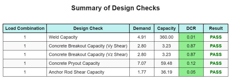
Résumé de la conception
Ce logiciel Logiciel de conception de plaques de base Skyciv peut générer automatiquement un rapport de calcul étape par étape pour cet exemple de conception. Il fournit également un résumé des contrôles effectués et de leurs ratios résultants, rendre les informations faciles à comprendre en un coup d'œil. Vous trouverez ci-dessous un échantillon de tableau de résumé, qui est inclus dans le rapport.
Rapport d'échantillon de skyciv
Découvrez le niveau de détail et de clarté que vous pouvez attendre d'un rapport de conception de plaque de base SkyCiv. Le rapport comprend toutes les vérifications de conception clés, équations, et les résultats présentés dans un format clair et facile à lire. Il est entièrement conforme aux normes de conception. Cliquez ci-dessous pour voir un exemple de rapport généré à l'aide du calculateur de plaque de base SkyCiv.
Logiciel d'achat de plaques de base
Achetez la version complète du module de conception de la plaque de base seul sans aucun autre module Skyviv. Cela vous donne un ensemble complet de résultats pour la conception de la plaque de base, y compris des rapports détaillés et plus de fonctionnalités.