Sistemas de lajes considerados pela norma
As normas australianas estabelecem os requisitos mínimos para o projeto de lajes de concreto armado, como tipos unidirecionais e bidirecionais. Sobre a configuração do plano e a inclusão de vigas, as lajes também podem ser divididas em lajes apoiadas em quatro lados, sistemas de vigas e lajes, lajes planas, e placas planas. Esses tipos estão resumidos nas imagens a seguir.
Simplifique a conformidade do projeto de laje australiana com o avançado SkyCiv exemplo-relatório-concreto. Experimente! Aplique AS facilmente 3600 verificações de lajes e placas planas.
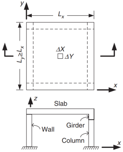
Figura 1. Laje apoiada nos quatro lados. (Yew-Chaye Loo & Abraço Sanual Chowdhury , “Concreto Armado e Protendido”, 22ª edição, Cambridge University Press).
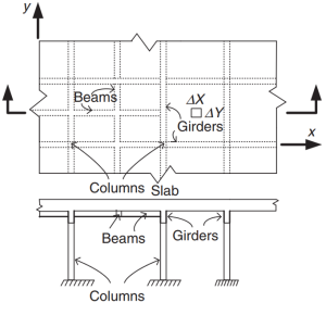
Figura 2. Sistema de laje de grelha. (Yew-Chaye Loo & Abraço Sanual Chowdhury , “Concreto Armado e Protendido”, 22ª edição, Cambridge University Press).
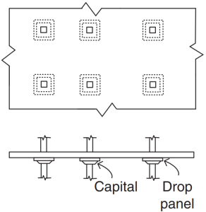
Figura 3. Lajes Planas. (Yew-Chaye Loo & Abraço Sanual Chowdhury , “Concreto Armado e Protendido”, 22ª edição, Cambridge University Press).
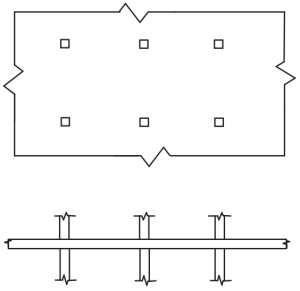
Figura 4. Placas Planas. (Yew-Chaye Loo & Abraço Sanual Chowdhury , “Concreto Armado e Protendido”, 22ª edição, Cambridge University Press).
A Norma recomenda alguns métodos (procedimentos simplificados e comprovados) na determinação dos momentos fletores:
- Cláusula 6.10.2: Vigas contínuas e lajes unidirecionais
- Cláusula 6.10.3: Lajes bidirecionais apoiadas nos quatro lados
- Cláusula 6.10.4: Lajes de duas vias com vários vãos
O objetivo do código é projetar a quantidade total de vergalhões de aço de reforço nas direções principais no sistema de laje. O aço do vergalhão será calculado para os momentos fletores “Mx” e “Meu.” Figura 5 mostra as demais forças ou ações em um elemento finito de laje em que a norma prescreve seus valores de resistência.
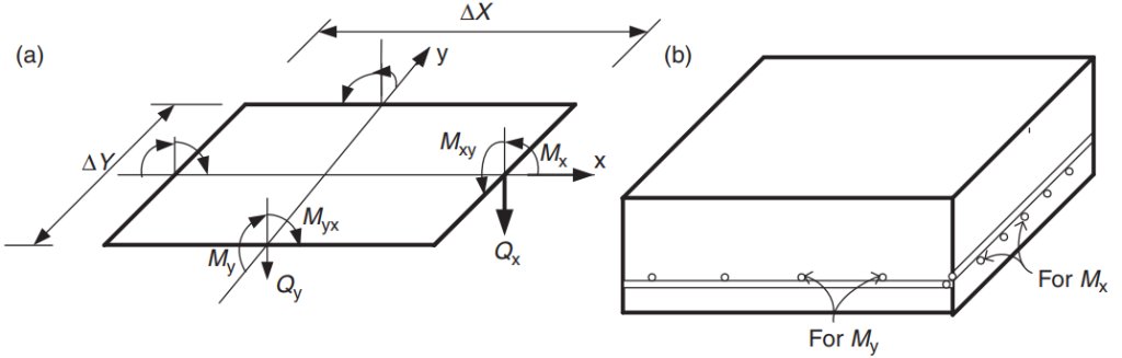
Figura 5. Forças em um elemento finito de laje: momentos de flexão (Mx, Minhas), momentos tortuosos (Mxy, Mix), e tesoura (Qx, Qy). (Yew-Chaye Loo & Abraço Sanual Chowdhury , “Concreto Armado e Protendido”, 22ª edição, Cambridge University Press)
Neste artigo, desenvolveremos dois exemplos de projeto de laje, sistemas de lajes unidirecionais e bidirecionais, usando os métodos simplificados orientados e permitidos pelo código. Em ambos os casos, criaremos um modelo SkyCiv S3D e compararemos os resultados com os métodos mencionados acima.
Se você é novo no SkyCiv, Inscreva-se e teste você mesmo o software!
Exemplo de projeto de laje unidirecional
Abaixo é mostrado o pequeno edifício e as lajes que projetaremos
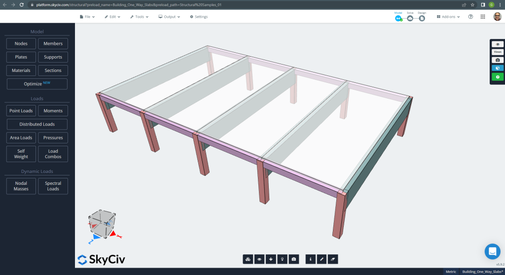
Figura 6. Exemplo de lajes unidirecionais em um pequeno edifício. (3D estrutural, Engenharia de Nuvem SkyCiv).
As dimensões do plano são mostradas a seguir
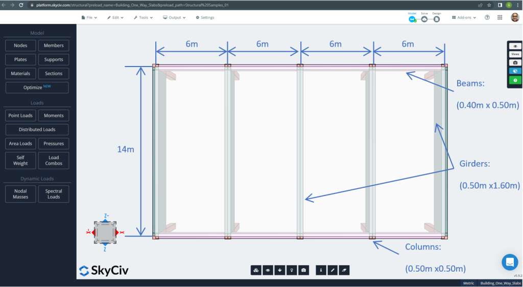
Figura 7. Dimensões do plano e elementos estruturais. (3D estrutural, Engenharia de Nuvem SkyCiv).
Para o exemplo de laje, resumindo, o material, propriedades dos elementos, e cargas a considerar :
- Classificação do tipo de laje: Um – comportamento de maneira \(\fratura{L_2}{L_1} > 2 ; \fratura{14m}{6m}=2,33 > 2.00 \) OK!
- ocupação do edifício: Uso residencial
- Espessura da laje \(t_{laje}=0.25m\)
- Densidade do concreto armado assumindo uma taxa de armadura de aço de 0.5% \(\rho_w = 24 \fratura{kN}{m^3} + 0.6 \fratura{kN}{m^3} \vezes 0.5 = 24.3 \fratura{kN}{m^3} \)
- Resistência à compressão característica do concreto em 28 dias \(f'c = 25 MPa \)
- Módulo de elasticidade do concreto pelo padrão australiano \(E_c = 26700 MPa \)
- Peso próprio da laje \(Dead = \rho_w \times t_{laje} = 24.3 \fratura{kN}{m^3} \vezes 0,25m = 6.075 \fratura {kN}{m^2}\)
- Carga morta superimposta \(SD = 3.0 \fratura {kN}{m^2}\)
- Carga viva \(L = 2.0 \fratura {kN}{m^2}\)
Cálculo manual de acordo com a norma AS3600
Nesta secção, calcularemos o vergalhão de aço reforçado necessário usando a referência do padrão australiano. Primeiro obtemos o momento fletor fatorado total a ser realizado pela faixa de largura unitária da laje.
- Carga morta, \(g = (3.0 + 6.075) \fratura{kN}{m^2} \vezes 1 m = 9.075 \fratura{kN}{m}\)
- Carga viva, \(q = (2.0) \fratura{kN}{m^2} \vezes 1 m = 2.0 \fratura{kN}{m}\)
- carga final, \(Fd = 1.2\times g + 1.5\vezes q = (1.2\vezes 9.075 + 1.5\vezes 2.0)\fratura{kN}{m} =13.89 \frac{kN}{m} \)
Usando o método simplificado especificado pela norma, primeiro, é obrigatório cumprir as seguintes restrições:
- \(\fratura{L_i}{L_j} \a 1.2 . \fratura{6m}{6m} A seguir estão as diferentes maneiras de determinar os coeficientes de pressão de terra para calcular a resistência ao atrito unitária de estacas em areia < 1.2 \). OK!
- A carga deve ser uniforme. OK!
- \(q \le 2g. q=2 \frac{kN}{m} < 18.15 \fratura{kN}{m}\). OK!
- A seção transversal da laje deve ser uniforme. OK!.
Espessura mínima recomendada, d
\(d \ge \frac{EU_{fe}}{{k_3}{k_4}{\sqrt[3]{\fratura{\fratura{\Delta}{EU_{ef}}{E_c}}{F_{d, ef}}}}}\)
Onde
- \(k_3 = 1.0; k_4 = 1.75 \)
- \(\fratura{\Delta}{EU_{ef}}=1/250 \)
- \(E_c = 27600 MPa \)
- \(F_{d,ef} = (1.0 +inclui cálculos detalhados passo a passo{cs})\vezes g + (\psi_s + inclui cálculos detalhados passo a passo{cs}\times \psi_1) \vezes q =(1.0+0.8)\vezes 9.075 + (0.7+0.8\vezes 0.4)\vezes 2 = 18.375 kPa )
- \(\psi_s = 0.7 \) Fator de curto prazo de carga ativa
- \(\psi_1 = 0.4 \) Fator de carga ativa de longo prazo
- \(inclui cálculos detalhados passo a passo{cs} = 0.8 \)
\(d \ge \frac{5.50m}{{1.0}\vezes {1.75}{\sqrt[3]{\fratura{\fratura{1}{250}\vezes{27600 \vezes 10 ^ 3 kPa}}{18.375 kPa }}}} \ge 0,173m. d = 0,25m > 0.173m \) OK!
Uma vez que demonstramos que as restrições são satisfeitas, o momento fletor é calculado usando a expressão: \(M=\alpha \times F_d \times L_n^2\) Onde \(\alpha\) é uma constante definida na figura a seguir.
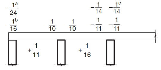
Figura 8. Valores do coeficiente de momento \(\alpha\) para lajes com mais de dois vãos. (Yew-Chaye Loo & Abraço Sanual Chowdhury , “Concreto Armado e Protendido”, 22ª edição, Cambridge University Press).
Onde:
- (uma) Caso de lajes e vigas apoiadas em viga
- (b) Somente para suporte de viga contínua
- (c) Onde o reforço Classe L é usado
- \(L_n \) é o vão unitário da faixa
- \(F_d \) é a carga fatorada gravitacional
Para o exemplo de laje, temos que usar o caso (uma) porque a laje repousa sobre vigas rígidas. Será explicado apenas um caso e o restante será mostrado na tabela a seguir. Incluímos também o cálculo da área de armadura de aço.
- \(M ={\alfa} {F_d}{L_n^2}={-\fratura{1}{24}}\vezes {13.89 \fratura{kN}{m}}\vezes (6m-0.5m)A partir da elevação do solo gerada a partir das elevações do Google – 17.51{kN}{m}\)
- Capa = 20mm (É necessário um mínimo de 10 mm para um período de resistência ao fogo de 60 minutos).
- \(d =t_{laje} – Cobrir – \fratura{Diâmetro da barra}{2} = 250 mm – 20milímetros – 6mm = 224 mm \)
- \(\alfa_2 = 1.0-0.003 f’c = 1.0-0.003\times 25 = 0.925 (0.67 \le \alpha_2 \le 0.85) \) Por isso, nós selecionamos \(\alfa_2 = 0.85\)
- \(\xi = \frac{\alpha_2\times f’c}{f_{seu}} = frac{0.85\vezes 25 MPa}{500 MPa} = 0.0425 \)
- \(\rho_t = \xi – \sqrt{{\XI}^ 2 – \fratura{{2}{\XI}{M}}{{\phi}{b}{d^2}{f_{seu}}}} = 0.0425 – \sqrt{{0.0425}^2-\frac{2\times 0.0425\times 17.51{kN}{m}}{{0.8}\vezes {1m}\vezes {{(0.224m)^ 2}} \vezes {500\vezes {10^ 3}kPa }}}=0.0008814\)
- \(\gama= 1.05-0.007 f’c = 1.05-0.007\times 25 = 0.875 (0.67 \le \gamma \le 0.85) \) Por isso, nós selecionamos \(\gama = 0.85\)
- \(k_u = \frac{\rho_t \times f_{seu}}{0.85\times \gamma \times f’c}= frac{0.0008814\vezes 500 MPa}{0.85\vezes 0.85 \vezes 25 MPa} =0.0244\)
- \(\phi = 1.19 – \fratura{13\inclui cálculos detalhados passo a passo{você0}}{12} = 1.19 – \fratura{13\vezes 0.0244}{12} = 1.164 (0.6 \le \phi \le 0.8) \) Por isso, nós selecionamos \(\phi = 0.8\). OK!.
- \(\rho_{t,min} = 0.20 {(\fratura{D}{d})^ 2}{(\fratura{f’_{ct,f}}{f_{seu}})} = 0.20 \vezes (\fratura{0.25m}{0.224m})^2 \times \frac{0.6\times sqrt{25MPa}}{500 MPa} = 0.0015\)
- \(UMA_{st}=max(\rho_{t,min}, \rho_t)\times b \times d = max(0.0015,0.0008814)\vezes 1000 mm \times 224 mm = 334.82 mm^2 \)
| \(\alpha\) e momentos | Exterior Negativo Esquerda | Exterior Positivo | Direita Negativa Externa | Interior Negativo Esquerda | Interior Positivo | Direito Negativo Interior |
|---|---|---|---|---|---|---|
| \(\alpha\) o Módulo de Young | -\(\fratura{1}{24}\) | \(\fratura{1}{11}\) | -\(\fratura{1}{10}\) | \(\fratura{1}{10}\) | \(\fratura{1}{16}\) | \(\fratura{1}{11}\) |
| valor M | -17.51 | 38.20 | -42.02 | 42.02 | 26.26 | 38.20 |
| \(\rho_t\) | 0.0008814 | 0.001948 | 0.002148 | 0.002148 | 0.00133 | 0.001948 |
| para | 0.0244 | 0.0539 | 0.0594 | 0.0594 | 0.0368 | 0.05391 |
| \(\phi) | 0.8 | 0.8 | 0.8 | 0.8 | 0.8 | 0.8 |
| \(UMA_{st} {mm^2}\) | 334.82 | 436.31 | 481.099 | 481.099 | 334.8214 | 436.3100 |
Após o cálculo da área do vergalhão de aço, você pode definir o detalhamento (a maneira real de colocar o reforço na laje). Como ajuda para o seu conhecimento, compartilhamos a seguinte imagem, que indica a localização do vergalhão para momentos positivos e negativos:
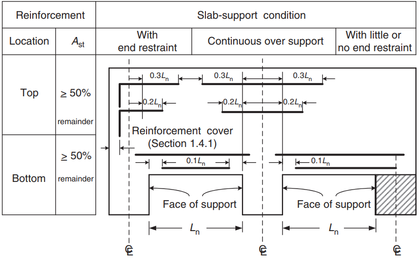
Figura 9. Arranjo de reforço para lajes unidirecionais e bidirecionais. (Yew-Chaye Loo & Abraço Sanual Chowdhury , “Concreto Armado e Protendido”, 22ª edição, Cambridge University Press)
Se você é novo no SkyCiv, Inscreva-se e teste você mesmo o software!
Resultados do Módulo de Projeto de Placa SkyCiv S3D
Na primeira vista, mostraremos algumas imagens para modelagem e análise estrutural do exemplo em S3D. Recomendamos que você leia sobre modelagem no SkyCiv nos links a seguir Como modelar placas? E Exemplo de design de laje ACI com SkyCiv.
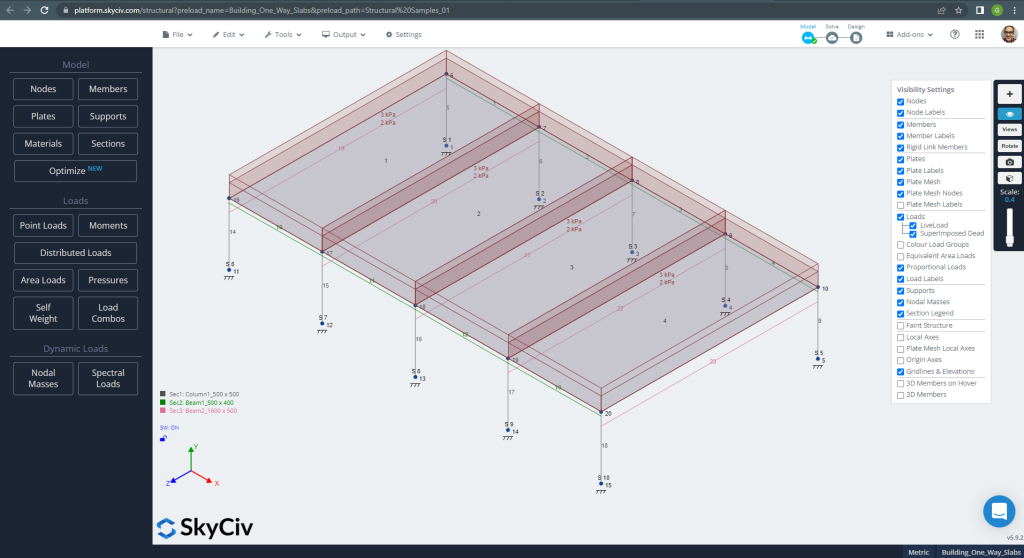
Figura 10. Exemplo de modelo estrutural em S3D para lajes unidirecionais. (3D estrutural, Engenharia de Nuvem SkyCiv).
Antes de analisar o modelo, devemos definir um tamanho de malha de placa. Algumas referências (2) recomendar um tamanho para o elemento shell de 1/6 do curto espaço ou 1/8 do longo vão, o mais curto deles. Seguindo este valor, temos \(\fratura{L2}{6}= frac{6m}{6} = 1 m \) ou \(\fratura{L1}{8}= frac{14m}{8}=1,75m \); tomamos 1m como tamanho máximo recomendado e 0,50m de tamanho de malha aplicado.
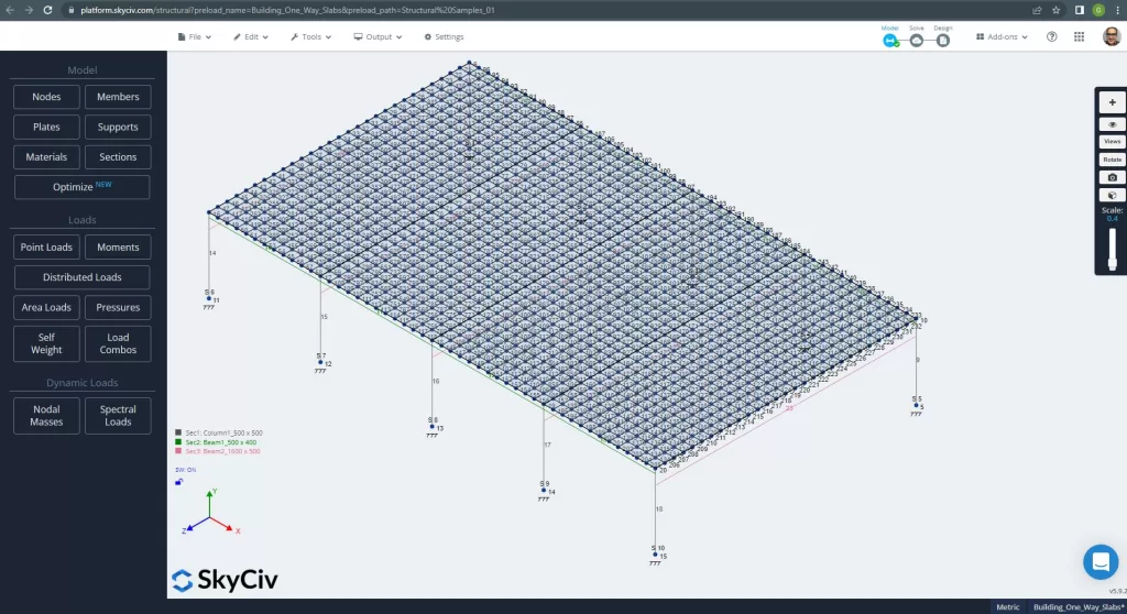
Figura 11. Malha aprimorada em placas. (3D estrutural, Engenharia de Nuvem SkyCiv).
Uma vez que melhoramos nosso modelo estrutural analítico, executamos uma análise elástica linear. Ao projetar lajes, temos que verificar se os deslocamentos verticais são menores que o máximo permitido pelo código. As Normas Australianas estabeleceram um deslocamento vertical máximo de manutenção de \(\fratura{L}{250}= frac{6000milímetros}{250}= 24,0 mm ).
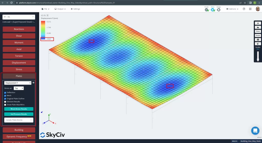
Figura 12. Deslocamento vertical em placas. (3D estrutural, Engenharia de Nuvem SkyCiv).
Comparando o deslocamento vertical máximo com o valor referenciado no código, a rigidez da laje é adequada. \(4.822 milímetros < 24.00mm ).
Os momentos máximos nos vãos da laje situam-se para positivo no centro e para negativo nos apoios exteriores e interiores. Vamos ver os valores desses momentos nas imagens a seguir.
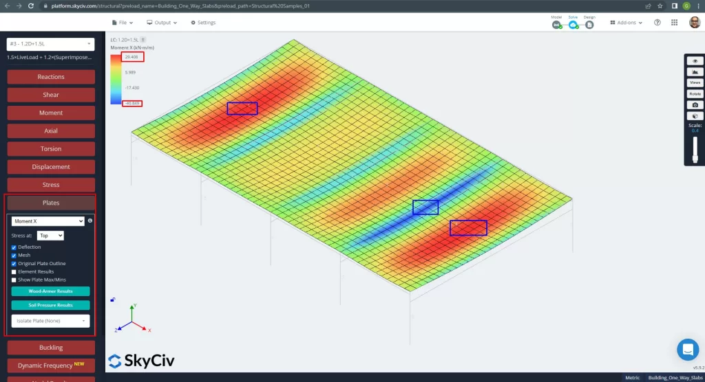
Figura 13. Momentos na direção X. (3D estrutural, Engenharia de Nuvem SkyCiv).
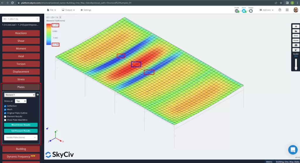
Figura 14. Momentos na direção Y. (3D estrutural, Engenharia de Nuvem SkyCiv).
Os eixos locais do elemento da placa são indicados abaixo.
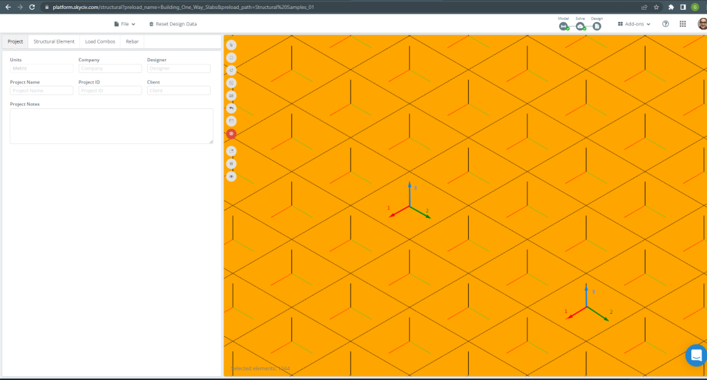
Figura 15. Eixos locais da laje. (3D estrutural, Engenharia de Nuvem SkyCiv).
Para mais detalhes sobre projeto automatizado de lajes armadas, veja nossa documentação Placas no SkyCiv.
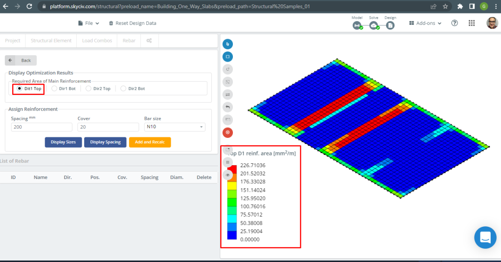
Figura 16. Reforço superior D1. (3D estrutural, Engenharia de Nuvem SkyCiv).
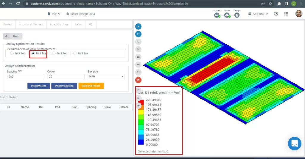
Figura 17. Reforço inferior D1. (3D estrutural, Engenharia de Nuvem SkyCiv).
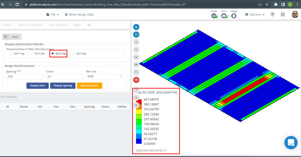
Figura 18. Reforço superior D2. (3D estrutural, Engenharia de Nuvem SkyCiv).
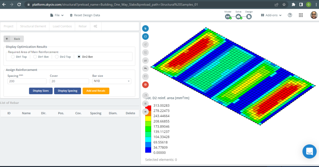
Figura 19. Reforço inferior D2. (3D estrutural, Engenharia de Nuvem SkyCiv).
Comparação de resultados
A última etapa neste exemplo de projeto de laje unidirecional é comparar a área do vergalhão de aço obtida pela análise S3D (eixos locais “2”) e cálculos manuais.
| Momentos e área de aço | Exterior Negativo Esquerda | Exterior Positivo | Direita Negativa Externa | Interior Negativo Esquerda | Interior Positivo | Direito Negativo Interior |
|---|---|---|---|---|---|---|
| \(UMA_{st, HandCalcs} {mm^2}\) | 334.82 | 436.31 | 481.099 | 481.099 | 334.8214 | 436.3100 |
| \(UMA_{st, S3D} {mm^2}\) | 285.13 | 313.00 | 427.69 | 427.69 | 313.00 | 427.69 |
| \(\Delta_{diferente}\) (%) | 14.84 | 28.262 | 11.101 | 11.101 | 6.517 | 1.986 |
Podemos ver que os resultados dos valores são muito próximos uns dos outros. Isso significa que os cálculos estão corretos!
Exemplo de projeto de laje de duas vias
Nesta secção, iremos desenvolver um exemplo que consiste em um sistema de grelha.
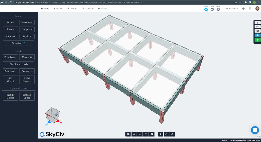
Figura 20. Sistema de grelha. (3D estrutural, Engenharia de Nuvem SkyCiv).
As dimensões do plano são mostradas a seguir
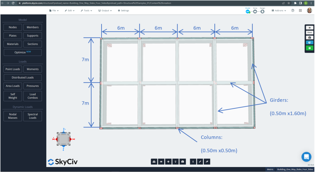
Figura 21. Exemplo de dimensões planejadas para o exemplo de laje bidirecional de quatro lados. (3D estrutural, Engenharia de Nuvem SkyCiv).
Para o exemplo de laje, resumindo, o material, propriedades dos elementos, e cargas a considerar :
- Classificação do tipo de laje: Dois – comportamento de maneira \(\fratura{L_2}{L_1} \a 2 ; \fratura{7m}{6m}=1,167 < 2.00 \) OK!
- ocupação do edifício: Uso residencial
- Espessura da laje \(t_{laje}=0.25m\)
- Densidade do concreto armado assumindo uma taxa de armadura de aço de 0.5% \(\rho_w = 24 \fratura{kN}{m^3} + 0.6 \fratura{kN}{m^3} \vezes 0.5 = 24.3 \fratura{kN}{m^3} \)
- Resistência à compressão característica do concreto em 28 dias \(f'c = 25 MPa \)
- Módulo de elasticidade do concreto pelo padrão australiano \(E_c = 26700 MPa \)
- Peso próprio da laje \(Dead = \rho_w \times t_{laje} = 24.3 \fratura{kN}{m^3} \vezes 0,25m = 6.075 \fratura {kN}{m^2}\)
- Carga morta superimposta \(SD = 3.0 \fratura {kN}{m^2}\)
- Carga viva \(L = 2.0 \fratura {kN}{m^2}\)
Cálculo manual de acordo com a norma AS3600
Nesta secção, calcularemos o vergalhão de aço reforçado necessário usando a referência do padrão australiano. Primeiro obtemos o momento fletor total fatorado a ser realizado pelas faixas de largura unitária da laje em cada direção principal de flexão.
- Carga morta, \(g = (3.0 + 6.075) \fratura{kN}{m^2} \vezes 1 m = 9.075 \fratura{kN}{m}\)
- Carga viva, \(q = (2.0) \fratura{kN}{m^2} \vezes 1 m = 2.0 \fratura{kN}{m}\)
- carga final, \(Fd = 1.2\times g + 1.5\vezes q = (1.2\vezes 9.075 + 1.5\vezes 2.0)\fratura{kN}{m} =13.89 \frac{kN}{m} \)
Momentos e coeficientes de projeto
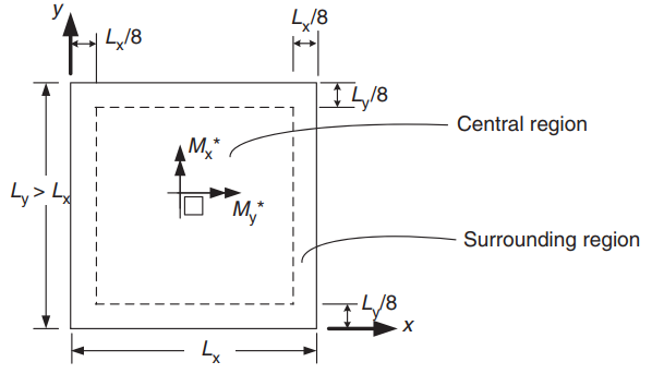
Figura 22. Orientação de uma laje bidirecional para determinação de momentos positivos. (Yew-Chaye Loo & Abraço Sanual Chowdhury , “Concreto Armado e Protendido”, 22ª edição, Cambridge University Press)
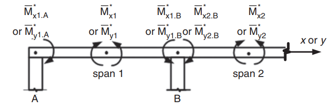
Figura 23. Determinação de momentos negativos em laje dupla. (Yew-Chaye Loo & Abraço Sanual Chowdhury , “Concreto Armado e Protendido”, 22ª edição, Cambridge University Press)
| Condição de borda | Coeficientes de curto vão (\(\beta_x\)) | Coeficientes de longo vão (\(\beta_y)\) todos os valores de \(\fratura{L_y}{L_x}\) | |||||||
|---|---|---|---|---|---|---|---|---|---|
| Valores de \(\fratura{L_y}{L_x}\) | |||||||||
| 1.0 | 1.1 | 1.2 | 1.3 | 1.4 | 1.5 | 1.75 | \(\cdot K_a 2.0\) | ||
| 1. Quatro arestas contínuas | 0.024 | 0.028 | 0.032 | 0.035 | 0.037 | 0.040 | 0.044 | 0.048 | 0.024 |
| 2. Uma borda curta descontínua | 0.028 | 0.032 | 0.036 | 0.038 | 0.041 | 0.043 | 0.047 | 0.050 | 0.028 |
| 3. Uma borda longa descontínua | 0.028 | 0.035 | 0.041 | 0.046 | 0.050 | 0.054 | 0.061 | 0.066 | 0.028 |
| 4. Duas bordas curtas descontínuas | 0.034 | 0.038 | 0.040 | 0.043 | 0.045 | 0.047 | 0.050 | 0.053 | 0.034 |
| 5. Duas bordas longas descontínuas | 0.034 | 0.046 | 0.056 | 0.065 | 0.072 | 0.078 | 0.091 | 0.100 | 0.034 |
| 6. Duas arestas adjacentes descontínuas | 0.035 | 0.041 | 0.046 | 0.051 | 0.055 | 0.058 | 0.065 | 0.070 | 0.035 |
| 7. Três arestas descontínuas (uma borda longa contínua) | 0.043 | 0.049 | 0.053 | 0.057 | 0.061 | 0.064 | 0.069 | 0.074 | 0.043 |
| 8. Três arestas descontínuas (uma borda curta contínua) | 0.043 | 0.054 | 0.064 | 0.072 | 0.078 | 0.084 | 0.096 | 0.105 | 0.043 |
| 9. Quatro arestas descontínuas | 0.056 | 0.066 | 0.074 | 0.081 | 0.087 | 0.093 | 0.103 | 0.111 | 0.056 |
Tabela 1. (Yew-Chaye Loo & Abraço Sanual Chowdhury , “Concreto Armado e Protendido”, 22ª edição, Cambridge University Press)
A imagem a seguir explica todos os nove casos aos quais a tabela acima se refere
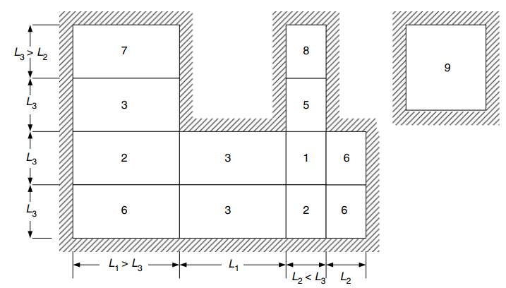
Figura 24. Condições de borda para lajes bidirecionais apoiadas em quatro lados. (Yew-Chaye Loo & Abraço Sanual Chowdhury , “Concreto Armado e Protendido”, 22ª edição, Cambridge University Press)
Momentos de design para região central (Caso 6 Duas arestas adjacentes descontínuas) :
- \(L_x = 6m, L_y=7m, \fratura{L_y}{L_x} = frac{7m}{6m}= 1.167 \) Valores a serem interpolados linearmente
- Positivos:
- \(M_x = {\beta_x}{F_d}{L_x^2} = {0.04435}\vezes {13.89 \fratura{kN}{m}}\vezes{(6m)^ 2}=22.177 kNm\)
- \(M_y = {\beta_y}{F_d}{L_x^2} ={0.035}\vezes {13.89 \fratura{kN}{m}}\vezes{(6m)^ 2}=17,501 kN·m \)
- Extensão externa negativa:
- \(M_{x1,A} = -\lambda_e \times M_x = -0.5 \vezes 22.177 kNm = – 11.089 kNm\)
- \(M_{y1,A} = -\lambda_e \times M_y = -0.5 \vezes 17.501 kNm = -8.751 kNm \)
- Vão interior negativo:
- \(M_{x1,B} = -\lambda_{1x} \vezes M_x = -1.33 \vezes 22.177 kNm = – 29.495 kNm\)
- \(M_{y1, B} = -\lambda_{1Y} \vezes M_y = -1.33 \vezes 17.501 kNm = -23.276 kNm \)
Momentos de design para região central (Caso 3 Uma borda longa descontínua) :
- \(L_x = 6m, L_y=7m, \fratura{L_y}{L_x} = frac{7m}{6m}= 1.167 \) Valores a serem interpolados linearmente
- Positivos:
- \(M_x = {\beta_x}{F_d}{L_x^2} = {0.03902}\vezes {13.89 \fratura{kN}{m}}\vezes{(6m)^ 2}= 19.512 kNm\)
- \(M_y = {\beta_y}{F_d}{L_x^2} ={0.028}\vezes {13.89 \fratura{kN}{m}}\vezes{(6m)^ 2}= 14.001 kNm \)
- Vão interior negativo:
- \(M_{x1,B} = -\lambda_{1x} \vezes M_x = -1.33 \vezes 19.512 kNm = – 25.951 kNm\)
- \(M_{y1, B} = -\lambda_{1Y} \vezes M_y = -1.33 \vezes 14.001 kNm = – 18.621 kNm \)
- Negativos dentro do segundo vão:
- \(M_{x2, B} = -\lambda_{2x} \vezes M_x = -1.33 \vezes 19.512 kNm = – 25.951 kNm\)
- \(M_{y2,B} = -\lambda_{2Y} \vezes M_y = -1.33 \vezes 14.001 kNm = – 18.621 kNm \)
Vergalhões de aço para direção X
| \(\alpha\) e momentos | Exterior Negativo Esquerda | Exterior Positivo | Direita Negativa Externa | Interior Negativo Esquerda | Interior Positivo | Direito Negativo Interior |
|---|---|---|---|---|---|---|
| valor M | 11.089 | 22.177 | 29.495 | 25.951 | 19.512 | 25.951 |
| \(\rho_t\) | 0.00055614 | 0.00112 | 0.001496 | 0.001313 | 0.000984 | 0.001313 |
| para | 0.015395 | 0.0310 | 0.0414 | 0.0364 | 0.0272 | 0.0364 |
| \(\phi) | 0.8 | 0.8 | 0.8 | 0.8 | 0.8 | 0.8 |
| \(UMA_{st} {mm^2}\) | 334.8214 | 334.8214 | 335.08233 | 334.821 | 334.8214 | 334.8214 |
Vergalhões de aço para direção Y
| \(\alpha\) e momentos | Exterior Negativo Esquerda | Exterior Positivo | Direita Negativa Externa | Interior Negativo Esquerda | Interior Positivo | Direito Negativo Interior |
|---|---|---|---|---|---|---|
| valor M | 8.751 | 17.501 | 23.276 | 18.621 | 14.001 | 18.621 |
| \(\rho_t\) | 0.0004383 | 0.0008811 | 0.001176 | 0.0009381 | 0.000703 | 0.0009381 |
| para | 0.0121 | 0.0244 | 0.03256 | 0.02597 | 0.0195 | 0.02597 |
| \(\phi) | 0.8 | 0.8 | 0.8 | 0.8 | 0.8 | 0.8 |
| \(UMA_{st} {mm^2}\) | 334.821 | 334.821 | 334.821 | 334.821 | 334.8214 | 334.821 |
Se você é novo no SkyCiv, Inscreva-se e teste você mesmo o software!
Resultados do Módulo de Projeto de Placa SkyCiv S3D
Depois de refinar o modelo, é hora de executar uma análise elástica linear.
Ao projetar lajes, temos que verificar se os deslocamentos verticais são menores que o máximo permitido pelo código. As Normas Australianas estabeleceram um deslocamento vertical máximo de manutenção de \(\fratura{L}{250}= frac{6000milímetros}{250}= 24,0 mm ).
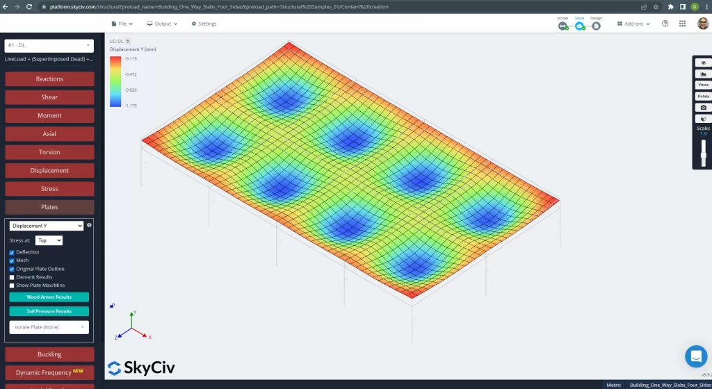
Figura 25. Deslocamento vertical no sistema de laje gradeada. (3D estrutural, Engenharia de Nuvem SkyCiv).
A imagem acima nos dá o deslocamento vertical. O valor máximo é de -1,179mm sendo inferior ao máximo permitido de -24mm. Portanto, a rigidez da laje é adequada.
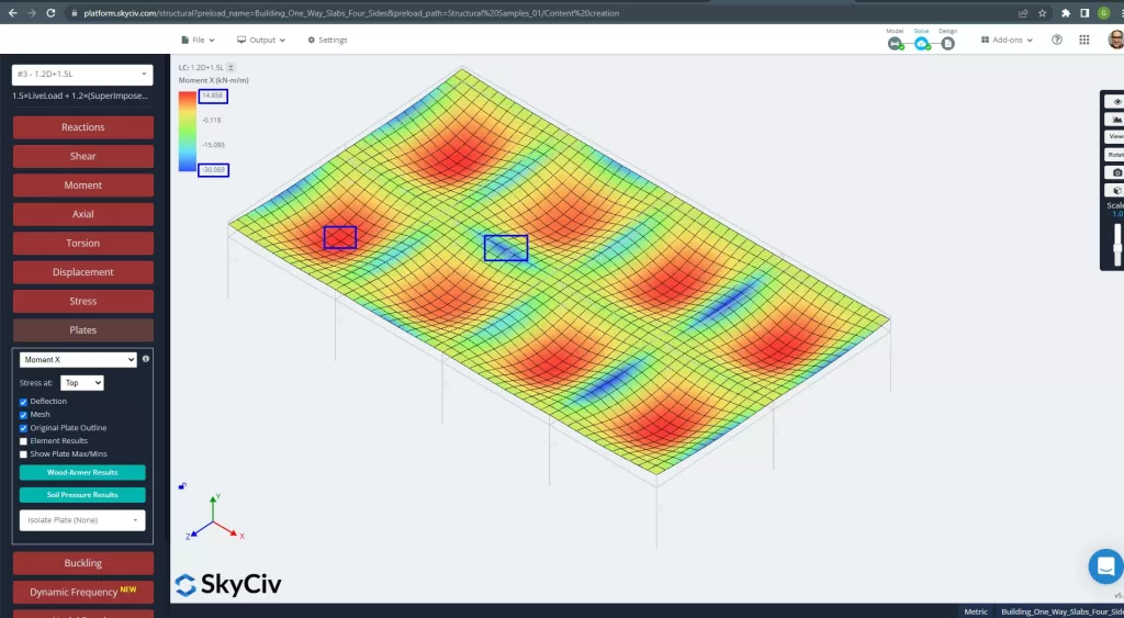
Figura 26. Momentos das placas na direção X. (3D estrutural, Engenharia de Nuvem SkyCiv).
Imagens 27 e 28 consistem no momento fletor em cada direção principal. Tomando a distribuição de momento e valores, o software, SkyCiv, pode-se obter então a área total da armadura de aço.
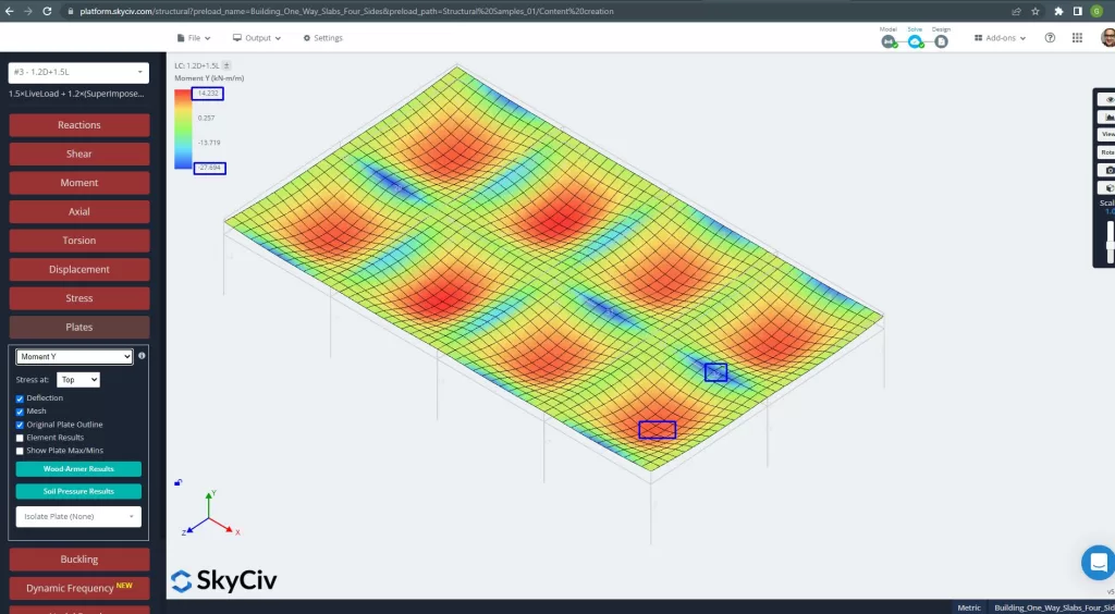
Figura 27. Momentos das placas na direção Y. (3D estrutural, Engenharia de Nuvem SkyCiv).
Áreas de reforço de aço:
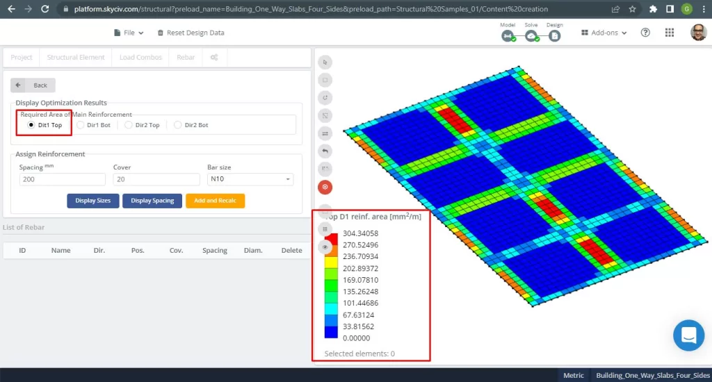
Figura 28. Reforço de vergalhão de aço superior na direção 1. (3D estrutural, Engenharia de Nuvem SkyCiv).
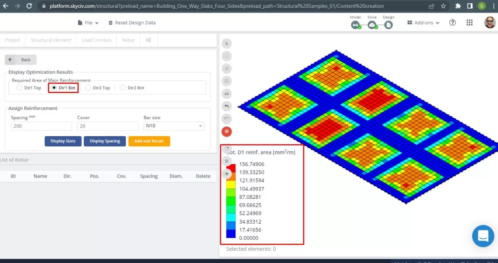
Figura 29. Reforço inferior do vergalhão de aço na direção 1. (3D estrutural, Engenharia de Nuvem SkyCiv).
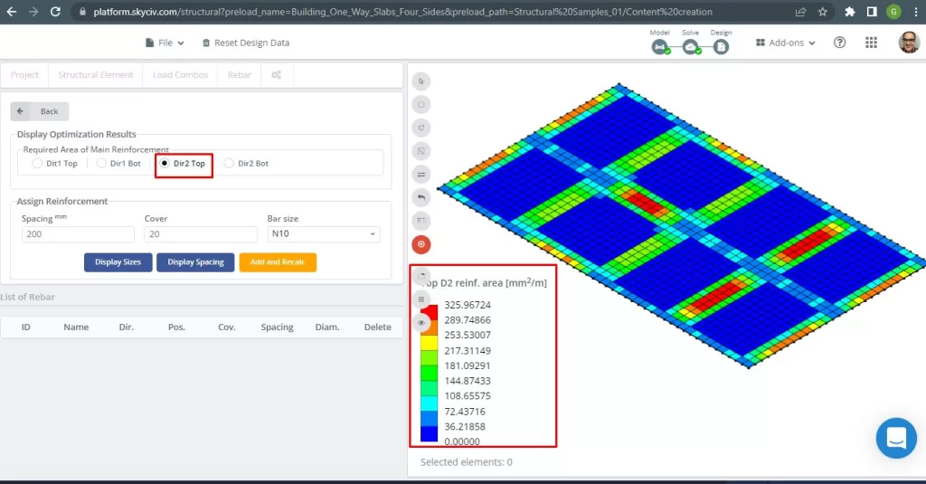
Figura 30. Reforço de vergalhão de aço superior na direção 2. (3D estrutural, Engenharia de Nuvem SkyCiv).
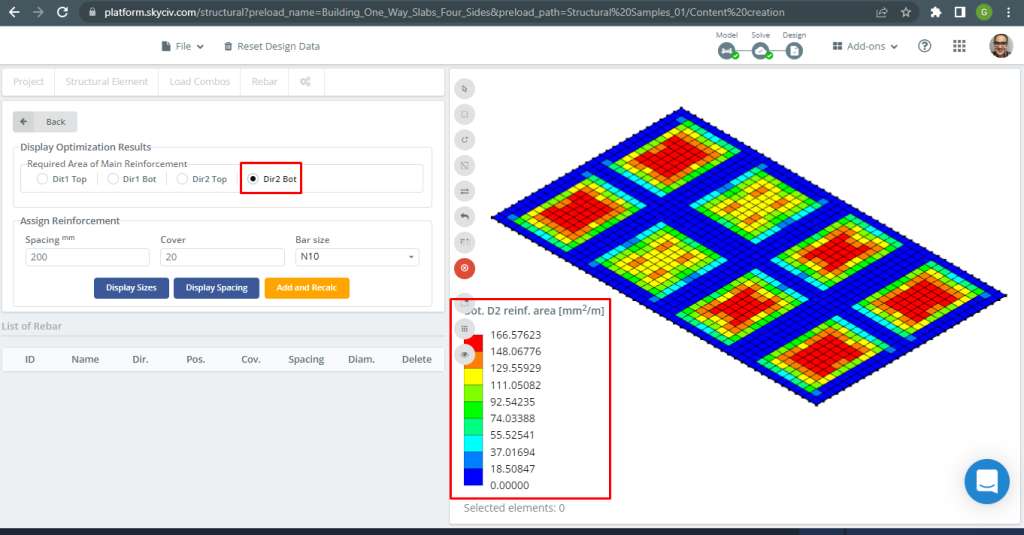
Figura 31. Reforço inferior do vergalhão de aço na direção 2. (3D estrutural, Engenharia de Nuvem SkyCiv).
Comparação de resultados
A última etapa neste exemplo de projeto de laje unidirecional é comparar a área do vergalhão de aço obtida pela análise S3D e cálculos manuais.
Vergalhões de aço para direção X
| Momentos e área de aço | Exterior Negativo Esquerda | Exterior Positivo | Direita Negativa Externa | Interior Negativo Esquerda | Interior Positivo | Direito Negativo Interior |
|---|---|---|---|---|---|---|
| \(UMA_{st, HandCalcs} {mm^2}\) | 334.8214 | 334.8214 | 335.08233 | 334.821 | 334.8214 | 334.8214 |
| \(UMA_{st, S3D} {mm^2}\) | 289.75 | 149.35 | 325.967 | 325.967 | 116.16 | 217.311 |
| \(\Delta_{diferente}\) (%) | 13.461 | 55.39 | 2.720 | 2.644 | 65.307 | 35.0964 |
Vergalhões de aço para direção Y
| Momentos e área de aço | Exterior Negativo Esquerda | Exterior Positivo | Direita Negativa Externa | Interior Negativo Esquerda | Interior Positivo | Direito Negativo Interior |
|---|---|---|---|---|---|---|
| \(UMA_{st, HandCalcs} {mm^2}\) | 334.821 | 334.821 | 334.821 | 334.821 | 334.821 | 334.821 |
| \(UMA_{st, S3D} {mm^2}\) | 270.524 | 156.75 | 304.34 | 304.34 | 156.75 | 270.52 |
| \(\Delta_{diferente}\) (%) | 19.203 | 53.184 | 9.104 | 9.104 | 53.184 | 19.204 |
A diferença é um pouco alta para momentos positivos e o motivo seria a presença de vigas com alta rigidez torcional que impactam nos resultados da Análise de Elementos Finitos de Placa e nos cálculos para armadura de flexão..
Se você é novo no SkyCiv, Inscreva-se e teste você mesmo o software!
Referências
- Yew-Chaye Loo & Abraço Sanual Chowdhury , “Concreto Armado e Protendido”, 22ª edição, Cambridge University Press.
- Bazan Enrique & Meli Piralla, “Projeto Sísmico de Estruturas”, 1ed, CLARO.
- Padrão Australiano, Estruturas de Concreto, AS 3600:2018