
No projeto de conexão de aço, parafusos geralmente são projetados como um grupo de parafusos que atua como um corpo para resistir a uma determinada carga. A resistência de um grupo de parafusos é normalmente definida pela resistência de controle do seu parafuso mais crítico.. As cargas diretas são distribuídas entre o número total de parafusos, enquanto o momento induzido devido à excentricidade da carga é distribuído em relação ao momento de inércia do grupo de parafusos e à distância do centroide. Isso é chamado de análise elástica. Devido às suas suposições simplificadas e conservadoras sobre distribuição de carga, muitas vezes produz conexões aparafusadas superdimensionadas.
Ao falar sobre engenharia de valor e projetos econômicos, a abordagem inelástica é preferida pela maioria dos fabricantes. Requer menos parafusos para a mesma magnitude de carga. Para fazer a abordagem inelástica, o centro instantâneo de rotação (ICOR) método usando iterações é a melhor maneira.
Neste artigo, demonstramos como calcular a força de um conexão parafusada usando o método ICOR. As reações por parafuso são calculadas usando a Equação (7-1) na página 7-7 do Manual AISC 15ª Edição. Isso é então usado para verificar se a localização assumida do centro instantâneo do grupo de parafusos está correta. Finalmente, assim que tivermos a localização correta do IC, calculamos o coeficiente do grupo de parafusos C para determinar sua resistência.
Trabalhado à mão, o método ICOR é um processo longo, porque encontrar o Centro Instantâneo (CI) é tentativa e erro. Com um solucionador de computador, o IC de um grupo de parafusos é encontrado por iterações programadas.. A SkyCiv Bolt Group Solver usa um método de iteração rápida para determinar a localização do IC e o coeficiente do grupo de parafusos em segundos. É usado tanto pelo AISC quanto pelo AS 4100 módulos de conexão.
O exemplo resolvido abaixo é o mesmo cálculo que o solucionador realiza, mostrado à mão longa para que você possa acompanhar o que está fazendo.
Obtendo as propriedades do grupo Bolt
Vamos começar com uma análise simples de um grupo de quatro parafusos carregados com uma carga de cisalhamento vertical excêntrica de 10 kips. A excentricidade da carga ao longo do eixo x é 4 polegadas à direita do grupo de parafusos. O ângulo da vertical é zero e a excentricidade ao longo do eixo y é zero.
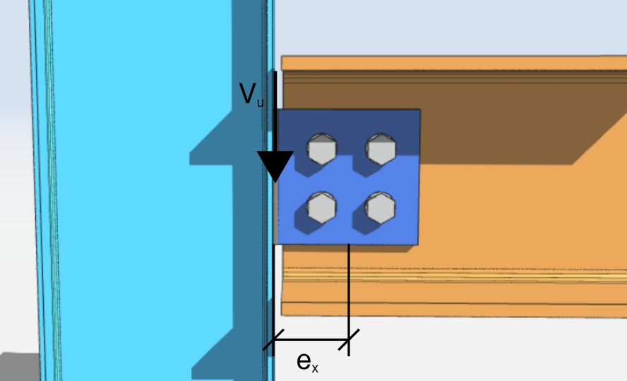
[math] V_{u} = 10\,kips [math]
[math] \theta = 0\,deg [math]
[math] e_{x} = 4\,in [math]
[math] e_{y} = 0\,in [math]
A primeira coisa a fazer é obter as coordenadas de todos os parafusos do grupo. Guias visuais e tabelas são altamente recomendados.
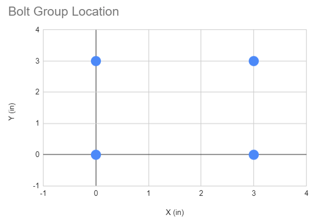
| Código da loja | X (no) | Y (no) |
| 1 | 0 | 0 |
| 2 | 0 | 3 |
| 3 | 3 | 0 |
| 4 | 3 | 3 |
Para obter o centróide do grupo de parafusos ao longo dos eixos x e y, precisamos da formula abaixo.
Deixar [mathin] n [mathin] = número total de parafusos
[math] X_{CG} = \frac{\sum X}{n} [math]
[math] Y_{CG} = \frac{\sum Y}{n} [math]
Então, nossa solução é:
[math] X_{CG} = \frac{\sum X}{n} = \frac{0\,in + 0\,in + 3\,in + 3\,in}{4} = 1.5\,in [math]
[math] Y_{CG} = \frac{\sum Y}{n} = \frac{0\,in + 3\,in + 0\,in + 3\,in}{4} = 1.5\,in [math]
Assuma a localização do I.C.
Depois de obter o centroide, assumimos a localização do centro instantâneo (CI). Como primeira tentativa, podemos assumir que o IC está no centróide geométrico do grupo de parafusos.
Então, presumir
[math] X_{IC} = X_{CG} = 1.5\,in [math]
[math] Y_{IC} = Y_{CG} = 1.5\,in [math]
Em seguida, tabulamos o deslocamento de cada parafuso do IC. Obtenha a distância ao longo de x e a distância ao longo de y primeiro, então o deslocamento resultante.
| Código da loja | cx (no) | cy (no) | c (no) |
| 1 | -1.5 | -1.5 | 2.121 |
| 2 | -1.5 | 1.5 | 2.121 |
| 3 | 1.5 | -1.5 | 2.121 |
| 4 | 1.5 | 1.5 | 2.121 |
Onde,
[math] c_{x} = X_{i} – X_{IC} [math]
[math] c_{y} = Y_{i} – Y_{IC} [math]
[math] c = \sqrt{ {\left( c_{x} \right)}^{2} + {\left( c_{y} \right)}^{2} } [math]
Para Parafuso Não. 1, nossa solução é
[math] c_{x} = 0\,in – 1.5\,in = -1.5\,in [math]
[math] c_{y} = 0\,in – 1.5\,in = -1.5\,in [math]
[math] c = \sqrt{ {\left( -1.5\,in \right)}^{2} + {\left( -1.5\,in \right)}^{2} } = 2.121\,in [math]
Calcule a deformação por parafuso wrt distância de IC
Depois de obter as distâncias dos parafusos do local assumido do IC, calculamos a deformação de cada parafuso em função de sua distância.
A deformação máxima por parafuso, [mathin] \Delta_{max} = 0.34\,in [mathin], é baseado em dados experimentais para um parafuso ASTM conforme descrito na página AISC 7-8. Por proporção linear, e configuração [mathin] \Delta_{max} = 0.34\,in [mathin], podemos calcular a deformação de um parafuso individual em relação à sua participação na distância máxima [mathin] c_{max} [mathin]. A equação para obter [mathin] \Delta [mathin] é mostrado abaixo.
[math] \Delta_{1} = 0.34\,in \times \left( \frac{c}{c_{max}} \right) [math]
Para Parafuso Não. 1, a deformação é
[math] \Delta_{1} = 0.34\,in \times \left( \frac{2.121\,in}{2.121\,in} \right) = 0.34\,in [math]
Porque o IC foi assumido no centróide, todos os quatro parafusos estão à mesma distância dele, então todos os quatro alcançam a mesma deformação. As deformações calculadas estão tabeladas abaixo.
| Código da loja | [mathin] \Delta [mathin] (no) |
| 1 | 0.34 |
| 2 | 0.34 |
| 3 | 0.34 |
| 4 | 0.34 |
Obtenha as reações por parafuso
Uma vez que temos a deformação por parafuso, usamos AISC 15ª Ed. Eq (7-1) para obter as reações por parafuso.
[math] R = R_{ult} \left( 1 – e^{-10\Delta} \right)^{0.55} [math]
A [mathin] R_{ult} [mathin] na equação é a carga última assumida em um parafuso, que podemos definir como a resistência ao cisalhamento do parafuso.
[math] R_{ult} = \phi R_{n} [math]
Para nosso exemplo, usamos uma resistência ao cisalhamento do parafuso de [mathin] 24.4\,kip [mathin]. Outro valor é igualmente válido, porque é cancelado quando calculamos o coeficiente do grupo de parafusos [mathin] C [mathin] mais tarde.
Para Parafuso Não. 1, a reação calculada é
[math] R = R_{ult} \left( 1 – e^{-10\Delta} \right)^{0.55} [math]
[math] R = 24.4\,kip \left( 1 – e^{-10 \times \left( 0.34\,in \right)} \right)^{0.55} [math]
[math] R = 23.949\,kip [math]
Para o resto dos parafusos, as reações calculadas são as seguintes. Os componentes da reação do parafuso [mathin] R [mathin] ao longo de x e y também são mostrados.
| Código da loja | R (kip) | Detalhes e parâmetros do modelo (kip) | Ry (kip) |
| 1 | 23.949 | 16.937 | -16.937 |
| 2 | 23.949 | -16.937 | -16.937 |
| 3 | 23.949 | 16.937 | 16.937 |
| 4 | 23.949 | -16.937 | 16.937 |
| ⅀Rx = 0 | ⅀Ry = 0 |
Cada força do parafuso atua perpendicularmente à linha que une esse parafuso ao IC, que é o que define o sinal de seus dois componentes. Para Parafuso Nº 1, as soluções para os componentes x e y são mostradas abaixo.
[math] R_{x} = -R \left( \frac{c_{y}}{c} \right) = -23.949 \times \left( \frac{-1.5\,in}{2.121\,in} \right) = 16.937\,kip [math]
[math] R_{y} = R \left( \frac{c_{x}}{c} \right) = 23.949 \times \left( \frac{-1.5\,in}{2.121\,in} \right) = -16.937\,kip [math]
Em seguida, precisamos do momento que cada reação do parafuso produz em relação ao IC. Use os componentes [mathin] R_{x} [mathin] e [mathin] R_{y} [mathin] com os braços de alavanca [mathin] c_{y} [mathin] e [mathin] c_{x} [mathin].
[math] M_{r} = -R_{x} c_{y} + R_{y} c_{x} [math]
Para Parafuso Nº 1, o momento de reação sobre o IC é
[math] M_{r} = -16.937\,kip \times \left( -1.5\,in \right) + \left( -16.937\,kip \right) \times \left( -1.5\,in \right) [math]
[math] M_{r} = 50.811\,kip\text{-}in [math]
Como um cheque, o mesmo momento é [mathin] R \times c = 23.949 \times 2.121 = 50.8\,kip\text{-}in [mathin], porque a força é perpendicular ao raio.
Cada parafuso aqui fica à mesma distância do CI assumido e carrega a mesma força, então cada parafuso retorna no mesmo momento. As reações de momento são tabeladas abaixo.
| Código da loja | Senhor (frango em) |
| 1 | 50.811 |
| 2 | 50.811 |
| 3 | 50.811 |
| 4 | 50.811 |
| ⅀Sr = 203.244 |
Verificando a localização do IC
Agora que temos as reações de cisalhamento e momento por parafuso, nós os usamos para determinar a carga que este grupo de parafusos resiste. Pegue a resultante da soma de todas as reações ao longo de x e a soma de todas as reações ao longo de y.
Da seção anterior, nós calculamos que
[math] \sum R_{x} = 0\,kip [math]
e
[math] \sum R_{y} = 0\,kip [math]
Então,
[math] P_{u} = \sqrt{ {\left( \sum R_{x} \right)}^{2} + {\left( \sum R_{y} \right)}^{2} } = 0\,kip [math]
A carga resultante é [mathin] P_{u} = 0\,kip [mathin]. Um grupo de parafusos girando em torno de seu próprio centróide carrega momento puro e nenhuma força resultante, então não pode resistir ao cisalhamento aplicado. Isso já nos diz que a primeira localização presumida do IC está errada, e poderíamos parar por aqui. Para o propósito desta discussão, continuaremos com as etapas restantes.
[math] P_{ux} = -P_{u}\sin\left( \theta \right) = 0\,kip [math]
[math] P_{uy} = -P_{u}\cos\left( \theta \right) = 0\,kip [math]
[math] M_{u} = -P_{ux}\left( Y_{CG} + e_{y} – Y_{IC} \right) + P_{uy} \left( X_{CG} + e_{x} – X_{IC} \right) = 0\,kip\text{-}in [math]
Desde a,
[math] P_{ux} \neq \sum R_{x} [math]
[math] P_{uy} \neq \sum R_{y} [math]
[math] M_{u} \neq \sum M_{r} [math]
O momento aplicado é zero enquanto as reações do parafuso somam 203.244 frango em, então o equilíbrio não é satisfeito. A localização presumida do I.C. está incorreto, e passamos para o próximo local assumido.
SkyCiv tem o cálculo do grupo de parafusos integrado em seus módulos de design de conexão. Quer experimentar nosso software de design de conexão?
Segunda Iteração
Para nossa segunda iteração, vamos assumir o I.C. está localizado nas coordenadas abaixo. Como a carga é um cisalhamento para baixo aplicado à direita do grupo, o verdadeiro IC fica à esquerda do centróide, então o julgamento se move nessa direção.
Presumir
[math] X_{IC} = 0.062\,in [math]
[math] Y_{IC} = 1.5\,in [math]
Em seguida, repita as etapas da primeira iteração. A tabela abaixo mostra as coordenadas, a distância de cada parafuso do I.C., e a deformação correspondente em relação a essa distância.
| Código da loja | X (no) | Y (no) | cx (no) | cy (no) | c (no) | [mathin] \Delta [mathin] (no) |
| 1 | 0 | 0 | -0.062 | -1.5 | 1.501 | 0.155 |
| 2 | 0 | 3 | -0.062 | 1.5 | 1.501 | 0.155 |
| 3 | 3 | 0 | 2.938 | -1.5 | 3.299 | 0.34 |
| 4 | 3 | 3 | 2.938 | 1.5 | 3.299 | 0.34 |
Desta vez, os parafusos não estão todos à mesma distância do IC, então apenas o par distante alcança o 0.34 no limite. O par próximo deforma menos e, portanto, carrega menos carga.
Observe que o centróide calculado do grupo de parafusos permanece inalterado, já que as coordenadas do parafuso não se moveram.
[math] X_{CG} = 1.5\,in [math]
[math] Y_{CG} = 1.5\,in [math]
Então calculamos as reações ao longo de x, as reações ao longo de y, e o momento correspondente. Os valores estão tabulados abaixo.
| Código da loja | R (kip) | Detalhes e parâmetros do modelo (kip) | Ry (kip) | Senhor (frango em) |
| 1 | 21.4 | 21.4 | -0.9 | 32.1 |
| 2 | 21.4 | -21.4 | -0.9 | 32.1 |
| 3 | 23.9 | 10.9 | 21.3 | 79.0 |
| 4 | 23.9 | -10.9 | 21.3 | 79.0 |
| ⅀Rx = 0 | ⅀Ry = 41 | ⅀Sr = 222 |
A continuação, determinamos a carga resultante de todas as reações ao longo de x e y.
[math] P_{u} = \sqrt{ {\left( \sum R_{x} \right)}^{2} + {\left( \sum R_{y} \right)}^{2} } [math]
[math] P_{u} = \sqrt{ {\left( 0\,kip \right)}^{2} + {\left( 40.703\,kip \right)}^{2} } [math]
[math] P_{u} = 40.703\,kip [math]
Então os componentes da carga resultante, com base no dado [mathin] \theta [mathin], são mostrados abaixo.
[math] P_{ux} = -P_{u}\sin\left( \theta \right) = -41\,kip \times \sin\left( 0\,deg \right) = 0\,kip [math]
[math] P_{uy} = -P_{u}\cos\left( \theta \right) = -41\,kip \times \cos\left( 0\,deg \right) = -41\,kip [math]
Em seguida, usamos esses componentes para resolver a carga de momento em torno do I.C assumido.
[math] M_{u} = -P_{ux} \left( Y_{CG} + e_{y} – Y_{IC} \right) + P_{uy} \left( X_{CG} + e_{x} – X_{IC} \right) [math]
[math] M_{u} = -0\,kip \left( 1.5\,in + 0\,in – 1.5\,in \right) + \left( -41\,kip \right) \left( 1.5\,in + 4\,in – 0.062\,in \right) [math]
[math] M_{u} = -222\,kip\text{-}in [math]
A continuação, vamos comparar o calculado [mathin] P_{ux} [mathin], [mathin] P_{uy} [mathin] e [mathin] M_{u} [mathin] contra as reações do grupo de parafusos.
[math] P_{ux} \approx -\sum R_{x} [math]
[math] P_{uy} \approx -\sum R_{y} [math]
[math] M_{u} \approx -\sum M_{r} [math]
Numericamente isso é 0 contra 0, -41 kip contra -41 kip, e -222 kip-in contra -222 frango em. O lado esquerdo está próximo o suficiente do lado direito para que possamos tomar a localização presumida do I.C.. tão correto.
Na prática, o solucionador continua movendo o IC de teste até que esses três resíduos caiam dentro de uma tolerância, em vez de parar em uma correspondência visual.
Resolvendo para o coeficiente C
Uma vez que o I. C.. a localização é determinada, podemos obter o coeficiente do grupo de parafusos C com a fórmula abaixo.
[math] C = \frac{P_{u}}{\phi R_{n}} = \frac{40.703\,kip}{24.4\,kip} = 1.668 [math]
O coeficiente significa que o grupo carrega 1.668 vezes a resistência de um único parafuso. Observe que isso está bem abaixo dos quatro parafusos presentes, porque a excentricidade custa ao grupo a maior parte da sua capacidade nominal. É também onde a escolha de [mathin] R_{ult} [mathin] cancela, é por isso que qualquer valor consistente pode ser usado no início.
Calculadora Gratuita de Grupo de Parafusos
Veja como projetamos nossas conexões parafusadas com esta abordagem no módulo de projeto de conexão. Escolha uma conexão parafusada, definir o layout do parafuso e a excentricidade, e o relatório fornece a localização do IC e o coeficiente C junto com todas as outras verificações. Ele roda no navegador, sem nada para instalar.
Para mais funcionalidade, incluindo salvar e recarregar seus arquivos, inscreva-se para uma conta gratuita.
