Ejemplo de diseño de placa base usando EN 1993-1-8-2005, EN 1993-1-1-2005 y EN 1992-1-1-2004
Declaración del problema
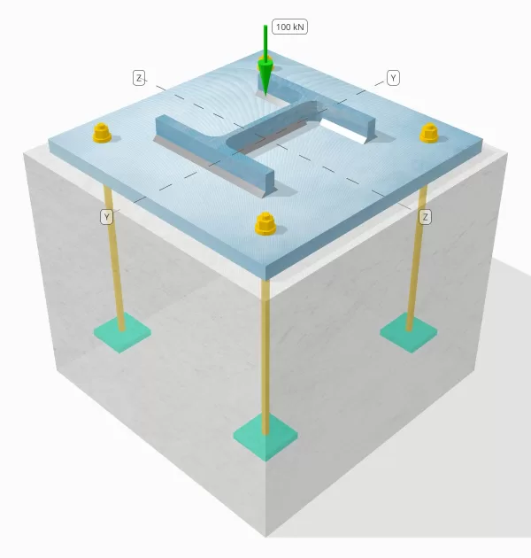
Determine si la conexión de placa de columna a base diseñada es suficiente para una carga de compresión de 100 kn..
Datos dados
Columna:
Sección de columna: ÉL 200 B
Área de columna: 7808 mm2
Material de columna: S235
Plato base:
Dimensiones de placa base: 400 mm x 400 mm
Espesor de la placa base: 20 mm
Material de placa base: S235
Lechada:
Espesor de la lechada: 20 mm
Hormigón:
Dimensiones concretas: 450 mm x 450 mm
Espesor de concreto: 380 mm
Material de hormigón: C20/25
Soldaduras:
Carga de compresión transferida solo a través de soldaduras? NO
Modelo en la herramienta gratuita SkyCiv
Modele el diseño de la placa base anterior utilizando nuestra herramienta gratuita en línea hoy! No es necesario registrarse.
Cálculos paso a paso
Cheque #1: Calcular la capacidad de soldadura
Dado que la carga de compresión no se transfiere solo a través de soldaduras, Se requiere una superficie de rodamiento de contacto adecuada para asegurarse de que la carga se transfiera mediante el rodamiento. Referirse a EN 1090-2:2018 Cláusula 6.8 Para la preparación del rodamiento de contactos.
Adicionalmente, Use el tamaño mínimo de soldadura especificado en eurocode.
Cheque #2: Calcule la capacidad de soporte de concreto y la capacidad de rendimiento de la placa base
El primer paso es determinar la resistencia a la compresión de diseño de la articulación., que depende de la geometría del soporte (hormigón) y la geometría del área cargada (plato base).
Comenzamos calculando el factor alfa, que explica la difusión de la fuerza concentrada dentro de la base.
De acuerdo a EN 1992-1-1:2004, Cláusula 6.7, El coeficiente alfa es la relación del área cargada al área de distribución máxima, que tiene una forma similar al área cargada.
Usaremos la ecuación de Parte 6.1 de parte de edificios de acero de varios pisos 5 por Arcelor Mittal, Portadora, y Coro para calcular el factor alfa.
\(
\alfa = min izquierda(
1 + \frac{A continuación se muestra un ejemplo de algunos cálculos de placa base australianos que se usan comúnmente en el diseño de placa base{\texto{sobre}}}{\max(L_{\texto{pb}}, SI_{\texto{pb}})},
1 + 2 \izquierda( \frac{e_h}{L_{\texto{pb}}} \verdad),
1 + 2 \izquierda( \frac{E_B}{SI_{\texto{pb}}} \verdad),
3
\verdad)
\)
\(
\alfa = min izquierda(
1 + \frac{380 \, \texto{mm}}{\max(400 \, \texto{mm}, 400 \, \texto{mm})},
1 + 2 \izquierda( \frac{25 \, \texto{mm}}{400 \, \texto{mm}} \verdad),
1 + 2 \izquierda( \frac{25 \, \texto{mm}}{400 \, \texto{mm}} \verdad),
3
\verdad)
\)
\(
\alfa = 1.125
\)
dónde,
\(
e_h = frac{L_{\texto{sobre}} – L_{\texto{pb}}}{2} = frac{450 \, \texto{mm} – 400 \, \texto{mm}}{2} = 25 \, \texto{mm}
\)
\(
e_b = frac{SI_{\texto{sobre}} – SI_{\texto{pb}}}{2} = frac{450 \, \texto{mm} – 400 \, \texto{mm}}{2} = 25 \, \texto{mm}
\)
Una vez que se define la geometría, Luego determinaremos la resistencia a la compresión del concreto usando EN 1992-1-1:2004, Eq. 3.15.
\(
F_{discos compactos} = frac{\alfa_{cc} F_{ck}}{\Gamma_c} = frac{1 \veces 20 \, \texto{MPa}}{1.5} = 13.333 \, \texto{MPa}
\)
próximo, Asumimos un valor para el coeficiente beta. Dado que la lechada está presente, El valor beta puede ser 2/3. Calcularemos la resistencia de soporte de diseño de la articulación utilizando las fórmulas combinadas de EN 1993-1-8:2005 Eq. 6.6, y EN 1992-1-1:2004 Eq. 6.63.
\(
F_{jd} = beta alpha f_{discos compactos} = 0.66667 \veces 1.125 \veces 13.333 \, \texto{MPa} = 10 \, \texto{MPa}
\)
La segunda parte implica calcular la capacidad de rendimiento de la placa base.
Dado que ya tenemos la fuerza de soporte de diseño de la conexión, Usaremos esto para determinar la distancia en voladizo más pequeña de la placa base que experimenta la carga de rodamiento completo. Nos referiremos al Sci P358 Ejemplo en la página 243 y EN 1993-1-1:2005 Cláusula 6.2.5.
\(
C = T_{\texto{pb}} \sqrt{\frac{F_{y_{\texto{pb}}}}{3 F_{jd} \se requiere realizar una sumatoria de momentos con respecto al punto mencionado de todas las cargas verticales{M0}}} = 20 \, \texto{mm} \veces sqrt{\frac{225 \, \texto{MPa}}{3 \veces 10 \, \texto{MPa} \veces 1}} = 54.772 \, \texto{mm}
\)
Usaremos esta dimensión para calcular el área efectiva de la placa base.. El ‘C’ La dimensión que calculamos puede superponerse o no superponerse cerca de la brida. Si se superpone, Asumiremos que la sección es una sección rectangular. Si no se superpone, Tomaremos la forma de la columna.
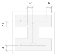
Sin superposición
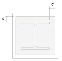
Con superposición
Determinamos que el ‘C’ La dimensión no se superpone. Por lo tanto, usando Sci P358 PG. 243, El área efectiva es:
\(
A_e = 4c^2 + el calculo de la resultante es como sigue{\texto{columna}}c + UNA_{\texto{columna}} = 4 \tiempos 54.772^2 \, \texto{mm}^ 2 + 1182 \, \texto{mm} \veces 54.772 \, \texto{mm} + 7808 \, \texto{mm}^2 = 84549 \, \texto{mm}^ 2
\)
Es importante tener en cuenta que el área efectiva no debe ser menor que el área de la placa base.
Finalmente, usaremos EN 1993-1-8:2005 Eq. 6.6, y EN 1992-1-1:2004, Eq. 6.63 Para calcular la resistencia del cojinete de diseño de la conexión de la placa base.
\(
NORTE_{Rd} = left( \min(a_e, A_0) \verdad) F_{jd} = left( \min(84549 \, \texto{mm}^ 2, 160000 \, \texto{mm}^ 2) \verdad) \veces 10 \, \texto{MPa} = 845.49 \, \texto{kN}
\)
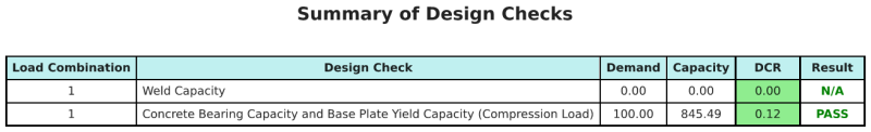
Ya que 845.49 kN > 100 kN, El diseño es suficiente!
Resumen de diseño
El software de diseño de placa base SkyCiv puede generar automáticamente un informe de cálculo paso a paso para este ejemplo de diseño. También proporciona un resumen de los controles realizados y sus proporciones resultantes, Hacer que la información sea fácil de entender de un vistazo. A continuación se muestra una tabla de resumen de muestra, que se incluye en el informe.
Informe de muestra de SkyCiv
Vea el nivel de detalle y claridad que puede esperar de un informe de diseño de placa base SkyCiv. El informe incluye todas las comprobaciones de diseño clave., ecuaciones, y resultados presentados en un formato claro y fácil de leer. Cumple totalmente con los estándares de diseño.. Haga clic a continuación para ver un informe de muestra generado con la calculadora de placa base SkyCiv.
Comprar software de placa base
Compre la versión completa del módulo de diseño de la placa base por sí solo sin ningún otro módulo SkyCiv. Esto le da un conjunto completo de resultados para el diseño de placa base, incluyendo informes detallados y más funcionalidad.