Sistemas de losas considerados por la norma
Normas australianas establecen los requisitos mínimos para el diseño de losas de hormigón armado, tales como tipos unidireccionales y bidireccionales. En cuanto a la configuración en planta y la inclusión de vigas, las losas también se pueden dividir en losas apoyadas en cuatro lados, sistemas de viga y losa, losas planas, y placas planas. Estos tipos se resumen en las siguientes imágenes..
Simplifique el cumplimiento del diseño de losas australianas con la tecnología avanzada de SkyCiv Software de diseño de estructuras de hormigón. Pruébalo! Aplicar AS fácilmente 3600 controles para losas y placas planas.
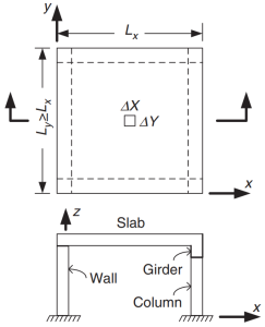
Figura 1. Losa apoyada en cuatro lados. (Yew-Chaye Loo & Sanual Abrazo Chowdhury , “Hormigón armado y pretensado”, 2segunda edición, Prensa de la Universidad de Cambridge).
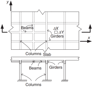
Figura 2. Sistema de losa de rejilla. (Yew-Chaye Loo & Sanual Abrazo Chowdhury , “Hormigón armado y pretensado”, 2segunda edición, Prensa de la Universidad de Cambridge).
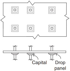
Figura 3. Losas Planas. (Yew-Chaye Loo & Sanual Abrazo Chowdhury , “Hormigón armado y pretensado”, 2segunda edición, Prensa de la Universidad de Cambridge).
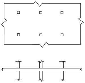
Figura 4. Platos Planos. (Yew-Chaye Loo & Sanual Abrazo Chowdhury , “Hormigón armado y pretensado”, 2segunda edición, Prensa de la Universidad de Cambridge).
La Norma recomienda algunos métodos (procedimientos simplificados y probados) en la determinación de los momentos flectores:
- Cláusula 6.10.2: Vigas continuas y losas en una dirección
- Cláusula 6.10.3: Losas en dos direcciones apoyadas en los cuatro lados
- Cláusula 6.10.4: Losas en dos direcciones de varios vanos
El propósito del código es diseñar la cantidad total de barras de refuerzo de acero en las direcciones principales en el sistema de losa.. Las barras de acero se calcularán para los momentos de flexión. “Mx” y “Mi.” Figura 5 muestra las otras fuerzas o acciones en un elemento de losa finito en el que el código prescribe sus valores de resistencia.
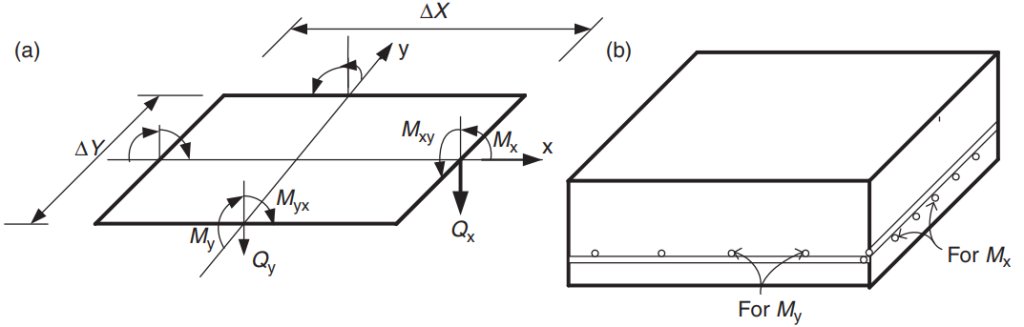
Figura 5. Fuerzas en un elemento de losa finito: momentos de flexión (Mx, Mi), momentos de torsión (Mxy, myx), y tijeras (Qx, Qy). (Yew-Chaye Loo & Sanual Abrazo Chowdhury , “Hormigón armado y pretensado”, 2segunda edición, Prensa de la Universidad de Cambridge)
En este artículo, desarrollaremos dos ejemplos de diseño de losas, sistemas de losas unidireccionales y bidireccionales, utilizando los métodos simplificados orientados y permitidos por el código. En ambos casos, crearemos un modelo SkyCiv S3D y compararemos los resultados con los métodos mencionados anteriormente.
Si eres nuevo en SkyCiv, Regístrese y pruebe el software usted mismo!
Ejemplo de diseño de losa en una dirección
A continuación se muestra el pequeño edificio y las losas que diseñaremos.
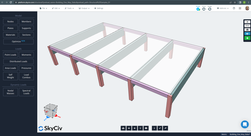
Figura 6. Ejemplo de losas unidireccionales en un edificio pequeño. (SkyCiv Estructural 3D , Ingeniería en la nube SkyCiv).
Las dimensiones del plano se muestran a continuación.
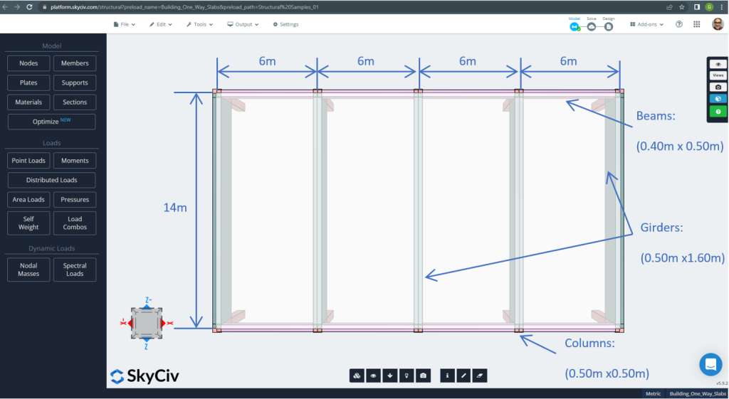
Figura 7. Dimensiones en planta y elementos estructurales. (SkyCiv Estructural 3D , Ingeniería en la nube SkyCiv).
Para el ejemplo de la losa, en resumen, el material, propiedades de los elementos, y mucho para considerar :
- Clasificación del tipo de losa: Uno – comportamiento de manera \(\frac{L_2}{L_1} > 2 ; \frac{14m}{6m}=2.33 > 2.00 \) OK!
- ocupación del edificio: uso residencial
- Espesor de losa \(A continuación se muestra un ejemplo de algunos cálculos de placa base australianos que se usan comúnmente en el diseño de placa base{losa}=0.25m)
- Densidad del hormigón armado suponiendo una relación de refuerzo de acero de 0.5% \(\rho_w = 24 \frac{kN}{m ^ 3} + 0.6 \frac{kN}{m ^ 3} \veces 0.5 = 24.3 \frac{kN}{m ^ 3} \)
- Resistencia característica a la compresión del hormigón a 28 dias \(f'c = 25 MPa \)
- Módulo de elasticidad del concreto según el estándar australiano \(E_c = 26700 MPa \)
- Peso propio de losa \(Muerto = rho_w times t_{losa} = 24.3 \frac{kN}{m ^ 3} \veces 0.25m = 6.075 \frac {kN}{m ^ 2}\)
- Carga muerta superpuesta \(DE = 3.0 \frac {kN}{m ^ 2}\)
- Carga viva \(L = 2.0 \frac {kN}{m ^ 2}\)
Cálculo manual según Norma AS3600
En esta sección, calcularemos la barra de refuerzo de acero reforzado requerida utilizando la referencia del estándar australiano. Primero se obtiene el momento flector mayorado total a realizar por la franja de ancho unitario de la losa.
- Peso muerto, \(g = (3.0 + 6.075) \frac{kN}{m ^ 2} \veces 1 m = 9.075 \frac{kN}{m}\)
- Carga viva, \(q = (2.0) \frac{kN}{m ^ 2} \veces 1 m = 2.0 \frac{kN}{m}\)
- Carga última, \(Fd = 1.2\times g + 1.5\veces q = (1.2\veces 9.075 + 1.5\veces 2.0)\frac{kN}{m} =13.89 \frac{kN}{m} \)
Utilizando el método simplificado especificado por la norma., primero, es obligatorio cumplir con las siguientes restricciones:
- \(\frac{L_i}{L_j} \la 1.2 . \frac{6m}{6m} =1 < 1.2 \). OK!
- La carga tiene que ser uniforme. OK!
- \(q le 2g. q=2 frac{kN}{m} < 18.15 \frac{kN}{m}\). OK!
- La sección transversal de la losa debe ser uniforme.. OK!.
Espesor mínimo recomendado, d
\(d ge frac{L_{fe}}{{k_3}{k_4}{\sqrt[3]{\frac{\frac{\Delta}{L_{ef}}{CE}}{F_{d, ef}}}}}\)
Dónde
- \(k_3 = 1.0; k_4 = 1.75 \)
- \(\frac{\Delta}{L_{ef}}=1/250 \)
- \(E_c = 27600 MPa \)
- \(F_{d,ef} = (1.0 +Suma de fuerzas de tensión de anclajes con área de cono de ruptura de concreto común{cs})\veces g + (\psi_s + Suma de fuerzas de tensión de anclajes con área de cono de ruptura de concreto común{cs}\veces psi_1) \veces q=(1.0+0.8)\veces 9.075 + (0.7+0.8\veces 0.4)\veces 2 = 18.375 kPa)
- \(\psi_s = 0.7 \) Factor de carga viva a corto plazo
- \(\psi_1 = 0.4 \) Factor de carga viva a largo plazo
- \(Suma de fuerzas de tensión de anclajes con área de cono de ruptura de concreto común{cs} = 0.8 \)
\(d ge frac{5.50m}{{1.0}\veces {1.75}{\sqrt[3]{\frac{\frac{1}{250}\veces{27600 \veces 10^3 kPa}}{18.375 kPa}}}} \edad 0.173m. d = 0,25 m > 0.173m \) OK!
Una vez demostramos que se satisfacen las restricciones, el momento de flexión se calcula mediante la expresión: \(M=\alpha \times F_d \times L_n^2\) dónde \(\alpha\) es una constante definida en la siguiente figura.
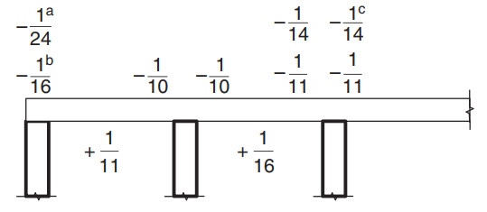
Figura 8. Valores del coeficiente de momento \(\alpha\) para losas de más de dos vanos. (Yew-Chaye Loo & Sanual Abrazo Chowdhury , “Hormigón armado y pretensado”, 2segunda edición, Prensa de la Universidad de Cambridge).
Dónde:
- (a) Caso de losas y vigas sobre apoyo de vigas
- (b) Solo para soporte de viga continua
- (c) Donde se usa refuerzo Clase L
- \(L_n \) es el tramo unitario de la tira
- \(F_d \) es la carga gravitatoria mayorada
Para el ejemplo de la losa, tenemos que usar el caso (a) porque la losa descansa sobre vigas rígidas. Se explicará un solo caso y el resto se mostrará en la siguiente tabla. Incluimos también el cálculo del área de refuerzo de acero.
- \(M={\alfa} {F_d}{L_n^2}={-\frac{1}{24}}\veces {13.89 \frac{kN}{m}}\veces (6m-0.5m)^2 = – 17.51{kN}{m}\)
- Cubierta = 20 mm (Se necesita un mínimo de 10 mm para un período de resistencia al fuego de 60 minutos).
- \(re = t_{losa} – Cubrir – \frac{BarDiámetro}{2} = 250 mm – 20mm – 6milímetro = 224 mm \)
- \(\alfa_2 = 1.0-0.003 f'c = 1,0-0,003veces 25 = 0.925 (0.67 \el alpha_2 el 0.85) \) Así, seleccionamos \(\alfa_2 = 0.85\)
- \(\xi = frac{\alpha_2veces f'c}{F_{su}} = frac{0.85\veces 25 MPa}{500 MPa} = 0.0425 \)
- \(\rho_t = xi – \sqrt{{\xi}^ 2 – \frac{{2}{\xi}{M}}{{\fi}{b}{re^2}{F_{su}}}} = 0.0425 – \sqrt{{0.0425}^2-frac{2\veces 0.0425veces 17.51{kN}{m}}{{0.8}\veces {1m}\veces {{(0.224m)^ 2}} \veces {500\veces {10^ 3}kPa}}}=0.0008814)
- \(\gamma= 1.05-0.007 f'c = 1,05-0,007veces 25 = 0.875 (0.67 \le gamma le 0.85) \) Así, seleccionamos \(\gama = 0.85\)
- \(k_u = frac{\rho_t veces f_{su}}{0.85\veces gamma veces f'c}= frac{0.0008814\veces 500 MPa}{0.85\veces 0.85 \veces 25 MPa} =0.0244)
- \(\fi = 1.19 – \frac{13\Suma de fuerzas de tensión de anclajes con área de cono de ruptura de concreto común{tu0}}{12} = 1.19 – \frac{13\veces 0.0244}{12} = 1.164 (0.6 \y phile 0.8) \) Así, seleccionamos \(\fi = 0.8\). OK!.
- \(\rho_{t,min} = 0.20 {(\frac{re}{d})^ 2}{(\frac{F'_{Connecticut,F}}{F_{su}})} = 0.20 \veces (\frac{0.25m}{0.224m})^2 \times \frac{0.6\veces sqrt{25MPa}}{500 MPa} = 0.0015\)
- \(UNA_{S t}= máx.(\rho_{t,min}, \rho_t)\times b \times d = max(0.0015,0.0008814)\veces 1000 mm \times 224 milímetro = 334.82 milímetro^2 \)
| \(\alpha\) y Momentos | Negativo Exterior Izquierdo | Positivo Exterior | Negativo Exterior Derecho | Interior Negativo Izquierdo | Interior Positivo | Interior Negativo Derecha |
|---|---|---|---|---|---|---|
| \(\alpha\) valor | -\(\frac{1}{24}\) | \(\frac{1}{11}\) | -\(\frac{1}{10}\) | \(\frac{1}{10}\) | \(\frac{1}{16}\) | \(\frac{1}{11}\) |
| valor M | -17.51 | 38.20 | -42.02 | 42.02 | 26.26 | 38.20 |
| \(\rho_t\) | 0.0008814 | 0.001948 | 0.002148 | 0.002148 | 0.00133 | 0.001948 |
| a | 0.0244 | 0.0539 | 0.0594 | 0.0594 | 0.0368 | 0.05391 |
| \(\fi) | 0.8 | 0.8 | 0.8 | 0.8 | 0.8 | 0.8 |
| \(UNA_{S t} {milímetro^2}\) | 334.82 | 436.31 | 481.099 | 481.099 | 334.8214 | 436.3100 |
Después del cálculo del área de la barra de acero, puedes definir los detalles (la forma real de colocar el refuerzo en la losa). Como ayuda para tu saber, compartimos la siguiente imagen, que indica la ubicación de la armadura para momentos positivos y negativos:
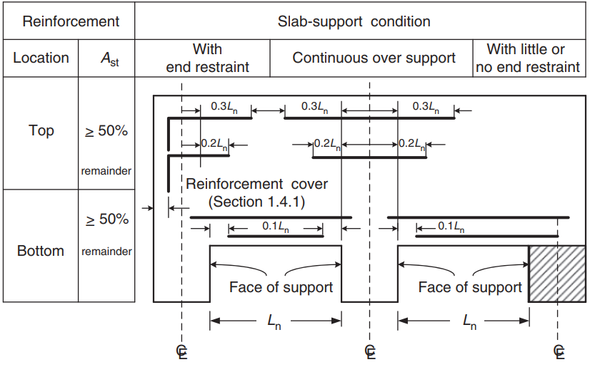
Figura 9. Arreglos de refuerzo para losas unidireccionales y bidireccionales. (Yew-Chaye Loo & Sanual Abrazo Chowdhury , “Hormigón armado y pretensado”, 2segunda edición, Prensa de la Universidad de Cambridge)
Si eres nuevo en SkyCiv, Regístrese y pruebe el software usted mismo!
Resultados del módulo de diseño de placas SkyCiv S3D
en la primera vista, mostraremos algunas imágenes para el modelado y análisis estructural del ejemplo en S3D. Te recomendamos leer sobre modelaje en SkyCiv en los siguientes enlaces Como modelar placas? Y Ejemplo de diseño de losa de ACI con SkyCiv.
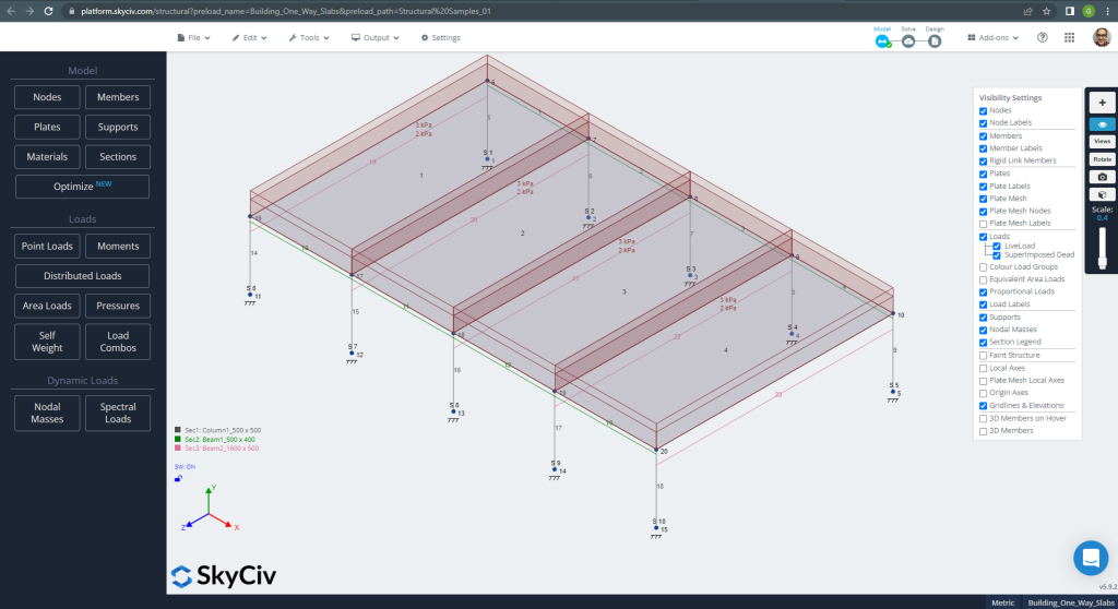
Figura 10. Modelo estructural en S3D para ejemplo de losas unidireccionales. (SkyCiv Estructural 3D , Ingeniería en la nube SkyCiv).
Antes de analizar el modelo, debemos definir un tamaño de malla de placa. Algunas referencias (2) recomendar un tamaño para el elemento shell de 1/6 del lapso corto o 1/8 del largo lapso, el más corto de ellos. Siguiendo este valor, tenemos \(\frac{L2}{6}= frac{6m}{6} = 1 metro \) o \(\frac{L1}{8}= frac{14m}{8}= 1,75 m \); tomamos 1 m como tamaño máximo recomendado y 0,50 m de malla aplicada.
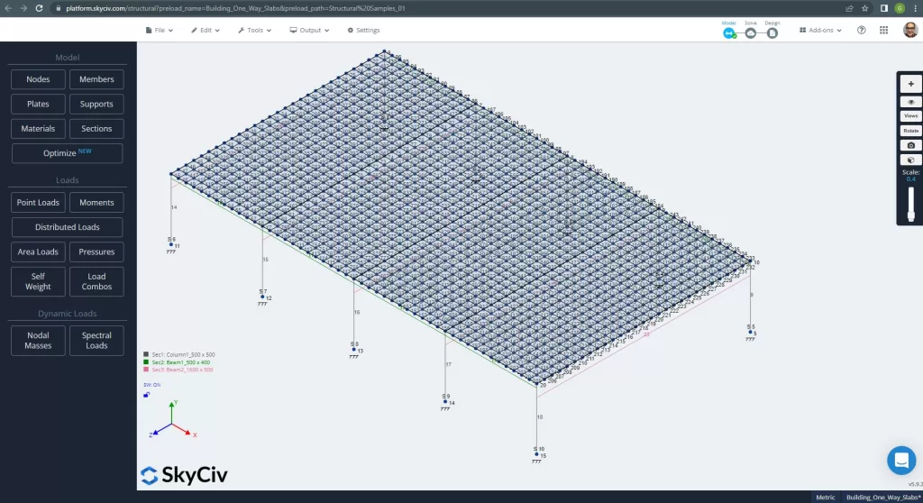
Figura 11. Malla mejorada en placas. (SkyCiv Estructural 3D , Ingeniería en la nube SkyCiv).
Una vez que mejoramos nuestro modelo estructural analítico, realizamos un análisis elástico lineal. Al diseñar losas, tenemos que comprobar si los desplazamientos verticales son inferiores al máximo permitido por el código. Las normas australianas establecieron un desplazamiento vertical máximo de servicio de \(\frac{L}{250}= frac{6000mm}{250}=24,0 mm).
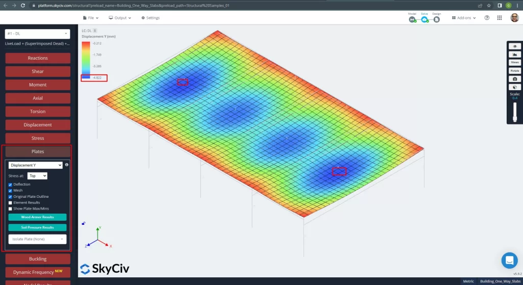
Figura 12. Desplazamiento vertical en placas. (SkyCiv Estructural 3D , Ingeniería en la nube SkyCiv).
Comparación del desplazamiento vertical máximo con el valor de referencia del código, la rigidez de la losa es adecuada. \(4.822 mm < 24.00mm).
Los momentos máximos en los vanos de la losa se ubican para positivo en el centro y para negativo en los apoyos exterior e interior.. Veamos los valores de estos momentos en las siguientes imágenes.
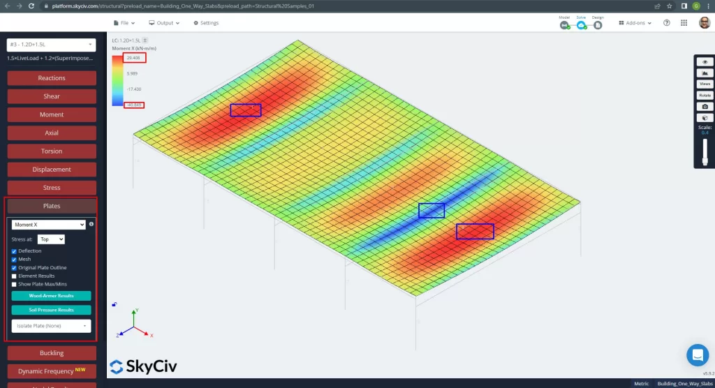
Figura 13. Momentos en la dirección X. (SkyCiv Estructural 3D , Ingeniería en la nube SkyCiv).
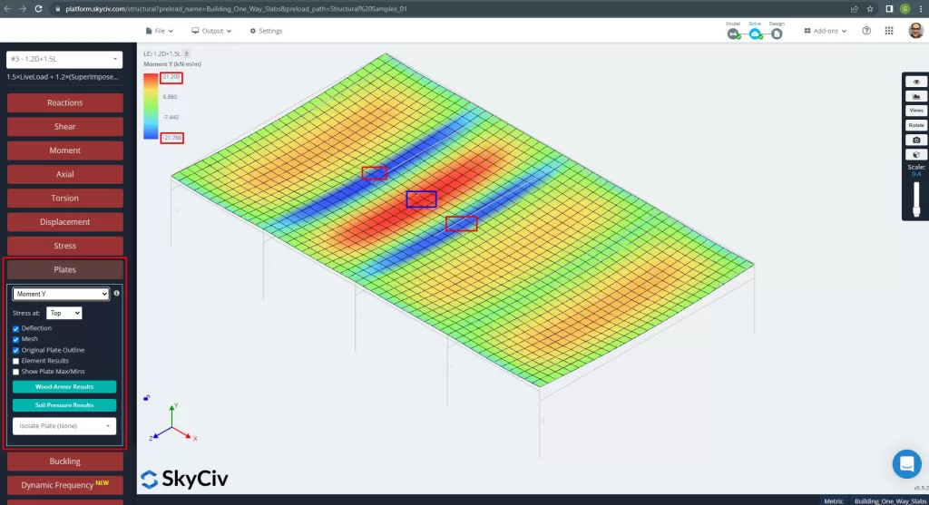
Figura 14. Momentos en la dirección Y. (SkyCiv Estructural 3D , Ingeniería en la nube SkyCiv).
Los ejes locales de los elementos de placa se indican a continuación..
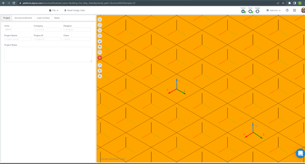
Figura 15. Ejes locales de losa. (SkyCiv Estructural 3D , Ingeniería en la nube SkyCiv).
Para más detalles sobre el diseño automatizado de losas armadas, ver nuestra documentación Placas en SkyCiv.
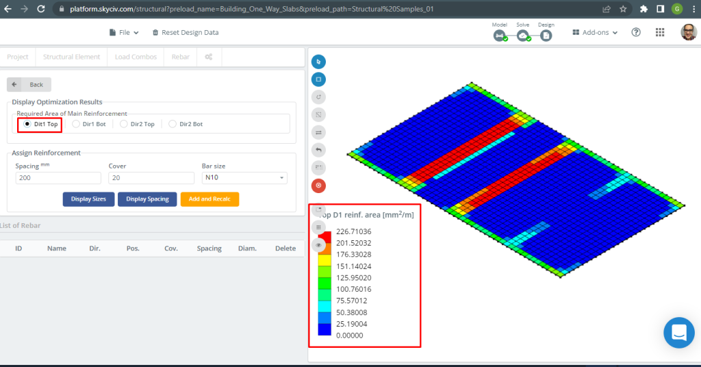
Figura 16. Refuerzo superior D1. (SkyCiv Estructural 3D , Ingeniería en la nube SkyCiv).
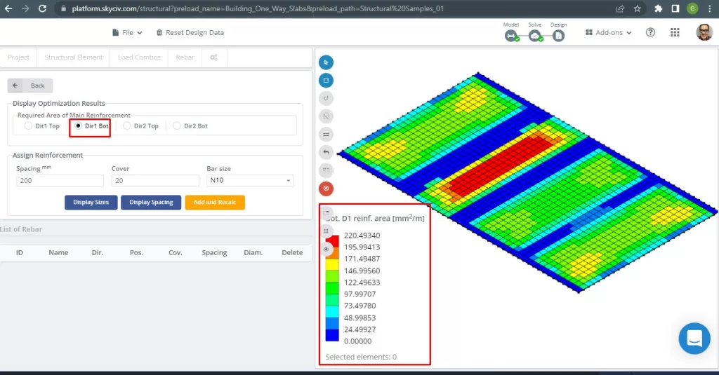
Figura 17. Refuerzo inferior D1. (SkyCiv Estructural 3D , Ingeniería en la nube SkyCiv).
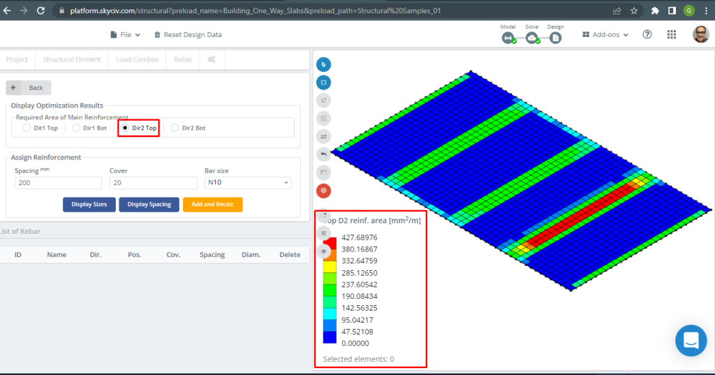
Figura 18. Refuerzo superior D2. (SkyCiv Estructural 3D , Ingeniería en la nube SkyCiv).
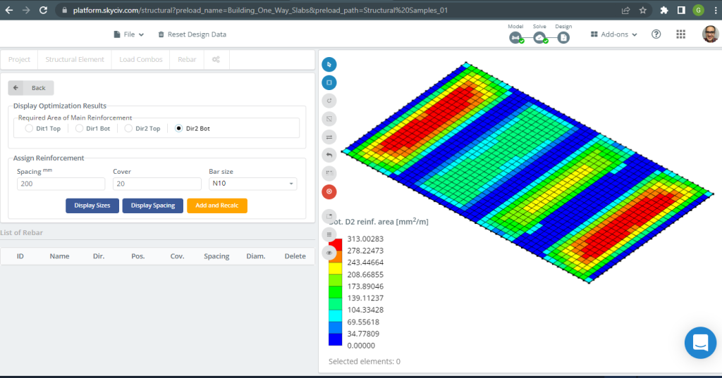
Figura 19. Refuerzo inferior D2. (SkyCiv Estructural 3D , Ingeniería en la nube SkyCiv).
Comparación de resultados
El último paso en este ejemplo de diseño de losa unidireccional es comparar el área de la barra de refuerzo de acero obtenida por análisis S3D (ejes locales “2”) y cálculos manuales.
| Momentos y área de acero | Negativo Exterior Izquierdo | Positivo Exterior | Negativo Exterior Derecho | Interior Negativo Izquierdo | Interior Positivo | Interior Negativo Derecha |
|---|---|---|---|---|---|---|
| \(UNA_{S t, Cálculos manuales} {milímetro^2}\) | 334.82 | 436.31 | 481.099 | 481.099 | 334.8214 | 436.3100 |
| \(UNA_{S t, S3D} {milímetro^2}\) | 285.13 | 313.00 | 427.69 | 427.69 | 313.00 | 427.69 |
| \(\Delta_{diferencia}\) (%) | 14.84 | 28.262 | 11.101 | 11.101 | 6.517 | 1.986 |
Podemos ver que los resultados de los valores están muy cerca uno del otro. Esto significa que los cálculos son correctos.!
Ejemplo de diseño de losa en dos direcciones
En esta sección, desarrollaremos un ejemplo que consiste en un sistema de rejilla.
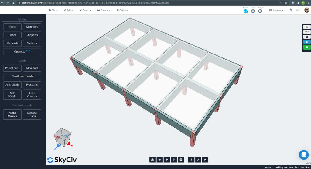
Figura 20. Sistema de parrilla. (SkyCiv Estructural 3D , Ingeniería en la nube SkyCiv).
Las dimensiones del plano se muestran a continuación.
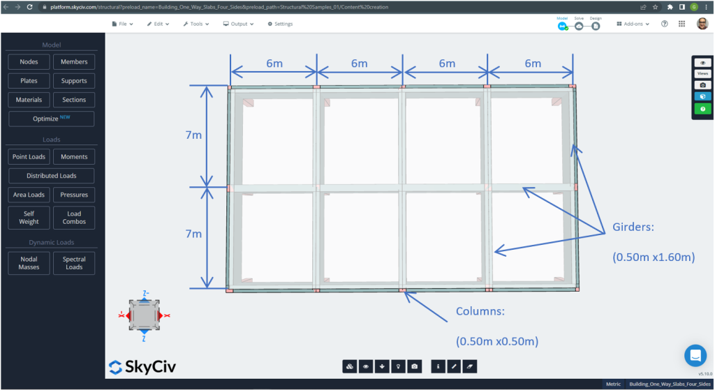
Figura 21. Dimensiones del plano para el ejemplo de losa en dos direcciones de cuatro lados. (SkyCiv Estructural 3D , Ingeniería en la nube SkyCiv).
Para el ejemplo de la losa, en resumen, el material, propiedades de los elementos, y mucho para considerar :
- Clasificación del tipo de losa: Dos – comportamiento de manera \(\frac{L_2}{L_1} \la 2 ; \frac{7m}{6m}=1.167 < 2.00 \) OK!
- ocupación del edificio: uso residencial
- Espesor de losa \(A continuación se muestra un ejemplo de algunos cálculos de placa base australianos que se usan comúnmente en el diseño de placa base{losa}=0.25m)
- Densidad del hormigón armado suponiendo una relación de refuerzo de acero de 0.5% \(\rho_w = 24 \frac{kN}{m ^ 3} + 0.6 \frac{kN}{m ^ 3} \veces 0.5 = 24.3 \frac{kN}{m ^ 3} \)
- Resistencia característica a la compresión del hormigón a 28 dias \(f'c = 25 MPa \)
- Módulo de elasticidad del concreto según el estándar australiano \(E_c = 26700 MPa \)
- Peso propio de losa \(Muerto = rho_w times t_{losa} = 24.3 \frac{kN}{m ^ 3} \veces 0.25m = 6.075 \frac {kN}{m ^ 2}\)
- Carga muerta superpuesta \(DE = 3.0 \frac {kN}{m ^ 2}\)
- Carga viva \(L = 2.0 \frac {kN}{m ^ 2}\)
Cálculo manual según Norma AS3600
En esta sección, calcularemos la barra de refuerzo de acero reforzado requerida utilizando la referencia del estándar australiano. Primero se obtiene el momento flector mayorado total a realizar por las tiras de ancho unitario de la losa en cada dirección principal de flexión.
- Peso muerto, \(g = (3.0 + 6.075) \frac{kN}{m ^ 2} \veces 1 m = 9.075 \frac{kN}{m}\)
- Carga viva, \(q = (2.0) \frac{kN}{m ^ 2} \veces 1 m = 2.0 \frac{kN}{m}\)
- Carga última, \(Fd = 1.2\times g + 1.5\veces q = (1.2\veces 9.075 + 1.5\veces 2.0)\frac{kN}{m} =13.89 \frac{kN}{m} \)
Momentos y coeficientes de diseño
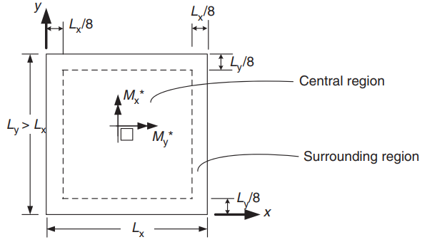
Figura 22. Orientación de una losa en dos direcciones para la determinación de momentos positivos. (Yew-Chaye Loo & Sanual Abrazo Chowdhury , “Hormigón armado y pretensado”, 2segunda edición, Prensa de la Universidad de Cambridge)
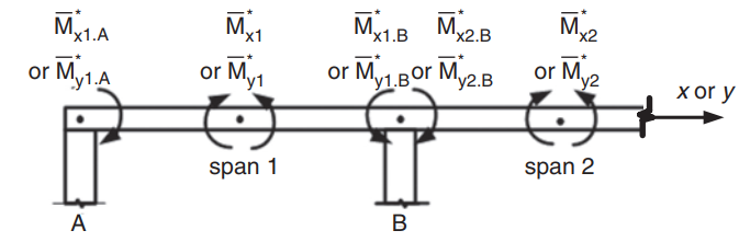
Figura 23. Determinación de momentos negativos en una losa en dos direcciones. (Yew-Chaye Loo & Sanual Abrazo Chowdhury , “Hormigón armado y pretensado”, 2segunda edición, Prensa de la Universidad de Cambridge)
| Condición de borde | Coeficientes de tramo corto (\(\beta_x)) | Coeficientes de tramo largo (\(\beta_y)\) todos los valores de \(\frac{L_y}{L_x}\) | |||||||
|---|---|---|---|---|---|---|---|---|---|
| Valores de \(\frac{L_y}{L_x}\) | |||||||||
| 1.0 | 1.1 | 1.2 | 1.3 | 1.4 | 1.5 | 1.75 | \(\La mitad de la altura de la pared desde la parte inferior de la base para el caso de la 2.0\) | ||
| 1. Cuatro aristas continuas | 0.024 | 0.028 | 0.032 | 0.035 | 0.037 | 0.040 | 0.044 | 0.048 | 0.024 |
| 2. Un borde corto discontinuos | 0.028 | 0.032 | 0.036 | 0.038 | 0.041 | 0.043 | 0.047 | 0.050 | 0.028 |
| 3. Un borde largo discontinuo | 0.028 | 0.035 | 0.041 | 0.046 | 0.050 | 0.054 | 0.061 | 0.066 | 0.028 |
| 4. Dos aristas cortas discontinuas | 0.034 | 0.038 | 0.040 | 0.043 | 0.045 | 0.047 | 0.050 | 0.053 | 0.034 |
| 5. Dos aristas largas discontinuas | 0.034 | 0.046 | 0.056 | 0.065 | 0.072 | 0.078 | 0.091 | 0.100 | 0.034 |
| 6. Dos aristas adyacentes discontinuas | 0.035 | 0.041 | 0.046 | 0.051 | 0.055 | 0.058 | 0.065 | 0.070 | 0.035 |
| 7. Tres aristas discontinuas (un borde largo continuo) | 0.043 | 0.049 | 0.053 | 0.057 | 0.061 | 0.064 | 0.069 | 0.074 | 0.043 |
| 8. Tres aristas discontinuas (un borde corto continuo) | 0.043 | 0.054 | 0.064 | 0.072 | 0.078 | 0.084 | 0.096 | 0.105 | 0.043 |
| 9. Cuatro aristas discontinuas | 0.056 | 0.066 | 0.074 | 0.081 | 0.087 | 0.093 | 0.103 | 0.111 | 0.056 |
Tabla 1. (Yew-Chaye Loo & Sanual Abrazo Chowdhury , “Hormigón armado y pretensado”, 2segunda edición, Prensa de la Universidad de Cambridge)
La siguiente imagen explica los nueve casos a los que se refiere la tabla anterior
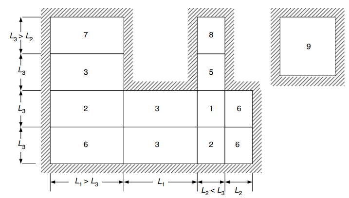
Figura 24. Condiciones de borde para losas en dos direcciones apoyadas en los cuatro lados. (Yew-Chaye Loo & Sanual Abrazo Chowdhury , “Hormigón armado y pretensado”, 2segunda edición, Prensa de la Universidad de Cambridge)
Momentos de diseño para la región central (Caso 6 Dos aristas adyacentes discontinuas) :
- \(L_x = 6m, L_y=7m, \frac{L_y}{L_x} = frac{7m}{6m}= 1.167 \) Valores a interpolar linealmente
- Positivos:
- \(M_x = {\beta_x}{F_d}{L_x^2} = {0.04435}\veces {13.89 \frac{kN}{m}}\veces{(6m)^ 2}=22.177 kNm\)
- \(M_y = {\beta_y}{F_d}{L_x^2} ={0.035}\veces {13.89 \frac{kN}{m}}\veces{(6m)^ 2}=17,501 kNm \)
- Luz exterior negativa:
- \(METRO_{x1,A} = -\lambda_e \times M_x = -0.5 \veces 22.177 kNm = – 11.089 kNm\)
- \(METRO_{y1,A} = -\lambda_e \times M_y = -0.5 \veces 17.501 kNm = -8.751 kNm \)
- Espacio interior negativo:
- \(METRO_{x1, segundo} = -lambda_{1x} \veces M_x = -1.33 \veces 22.177 kNm = – 29.495 kNm\)
- \(METRO_{y1, B} = -lambda_{1y} \veces M_y = -1.33 \veces 17.501 kNm = -23.276 kNm \)
Momentos de diseño para la región central (Caso 3 Un borde largo discontinuo) :
- \(L_x = 6m, L_y=7m, \frac{L_y}{L_x} = frac{7m}{6m}= 1.167 \) Valores a interpolar linealmente
- Positivos:
- \(M_x = {\beta_x}{F_d}{L_x^2} = {0.03902}\veces {13.89 \frac{kN}{m}}\veces{(6m)^ 2}= 19.512 kNm\)
- \(M_y = {\beta_y}{F_d}{L_x^2} ={0.028}\veces {13.89 \frac{kN}{m}}\veces{(6m)^ 2}= 14.001 kNm \)
- Espacio interior negativo:
- \(METRO_{x1, segundo} = -lambda_{1x} \veces M_x = -1.33 \veces 19.512 kNm = – 25.951 kNm\)
- \(METRO_{y1, B} = -lambda_{1y} \veces M_y = -1.33 \veces 14.001 kNm = – 18.621 kNm \)
- Negativos interior segundo vano:
- \(METRO_{x2,B} = -lambda_{2x} \veces M_x = -1.33 \veces 19.512 kNm = – 25.951 kNm\)
- \(METRO_{y2,B} = -lambda_{2y} \veces M_y = -1.33 \veces 14.001 kNm = – 18.621 kNm \)
Barra de acero para dirección X
| \(\alpha\) y Momentos | Negativo Exterior Izquierdo | Positivo Exterior | Negativo Exterior Derecho | Interior Negativo Izquierdo | Interior Positivo | Interior Negativo Derecha |
|---|---|---|---|---|---|---|
| valor M | 11.089 | 22.177 | 29.495 | 25.951 | 19.512 | 25.951 |
| \(\rho_t\) | 0.00055614 | 0.00112 | 0.001496 | 0.001313 | 0.000984 | 0.001313 |
| a | 0.015395 | 0.0310 | 0.0414 | 0.0364 | 0.0272 | 0.0364 |
| \(\fi) | 0.8 | 0.8 | 0.8 | 0.8 | 0.8 | 0.8 |
| \(UNA_{S t} {milímetro^2}\) | 334.8214 | 334.8214 | 335.08233 | 334.821 | 334.8214 | 334.8214 |
Barra de acero para dirección Y
| \(\alpha\) y Momentos | Negativo Exterior Izquierdo | Positivo Exterior | Negativo Exterior Derecho | Interior Negativo Izquierdo | Interior Positivo | Interior Negativo Derecha |
|---|---|---|---|---|---|---|
| valor M | 8.751 | 17.501 | 23.276 | 18.621 | 14.001 | 18.621 |
| \(\rho_t\) | 0.0004383 | 0.0008811 | 0.001176 | 0.0009381 | 0.000703 | 0.0009381 |
| a | 0.0121 | 0.0244 | 0.03256 | 0.02597 | 0.0195 | 0.02597 |
| \(\fi) | 0.8 | 0.8 | 0.8 | 0.8 | 0.8 | 0.8 |
| \(UNA_{S t} {milímetro^2}\) | 334.821 | 334.821 | 334.821 | 334.821 | 334.8214 | 334.821 |
Si eres nuevo en SkyCiv, Regístrese y pruebe el software usted mismo!
Resultados del módulo de diseño de placas SkyCiv S3D
Después de refinar el modelo, es hora de ejecutar un análisis elástico lineal.
Al diseñar losas, tenemos que comprobar si los desplazamientos verticales son inferiores al máximo permitido por el código. Las normas australianas establecieron un desplazamiento vertical máximo de servicio de \(\frac{L}{250}= frac{6000mm}{250}=24,0 mm).
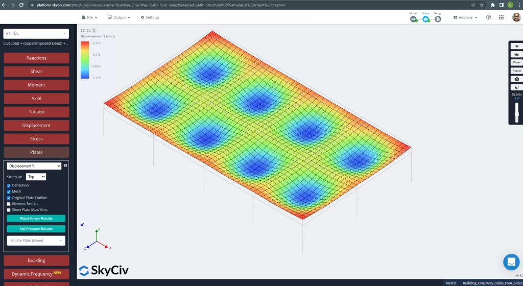
Figura 25. Desplazamiento vertical en el sistema de losa de emparrillado. (SkyCiv Estructural 3D , Ingeniería en la nube SkyCiv).
La imagen de arriba nos da el desplazamiento vertical.. El valor máximo es -1.179mm siendo menor que el máximo permitido de -24mm. Por lo tanto, la rigidez de la losa es adecuada.
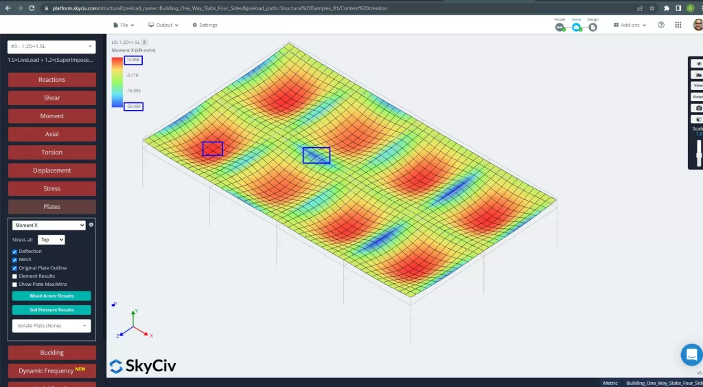
Figura 26. Momentos de las placas en la dirección X. (SkyCiv Estructural 3D , Ingeniería en la nube SkyCiv).
Imágenes 27 y 28 consisten en el momento de flexión en cada dirección principal. Tomando la distribución de momentos y valores, El software, SkyCiv, puede obtener entonces el área total de refuerzo de acero.
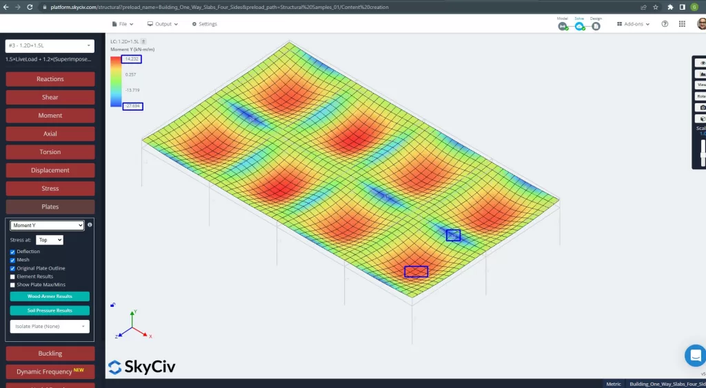
Figura 27. Momentos de las placas en la dirección Y. (SkyCiv Estructural 3D , Ingeniería en la nube SkyCiv).
Áreas de refuerzo de acero:
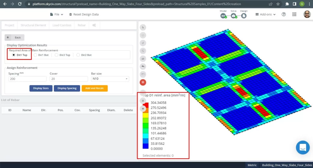
Figura 28. Refuerzo de barra de acero superior en dirección 1. (SkyCiv Estructural 3D , Ingeniería en la nube SkyCiv).
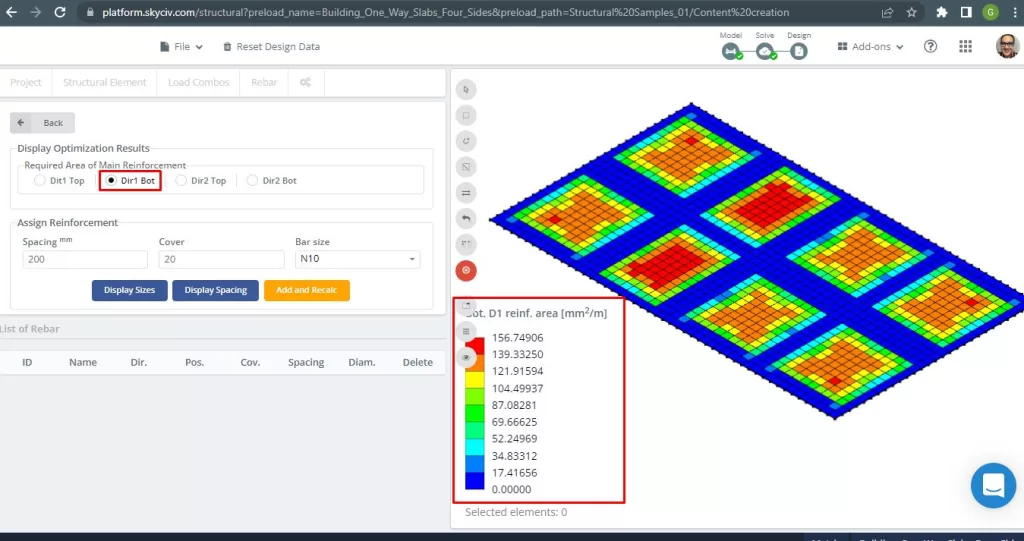
Figura 29. Refuerzo de barra de acero inferior en dirección 1. (SkyCiv Estructural 3D , Ingeniería en la nube SkyCiv).
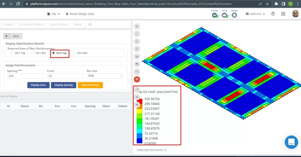
Figura 30. Refuerzo de barra de acero superior en dirección 2. (SkyCiv Estructural 3D , Ingeniería en la nube SkyCiv).
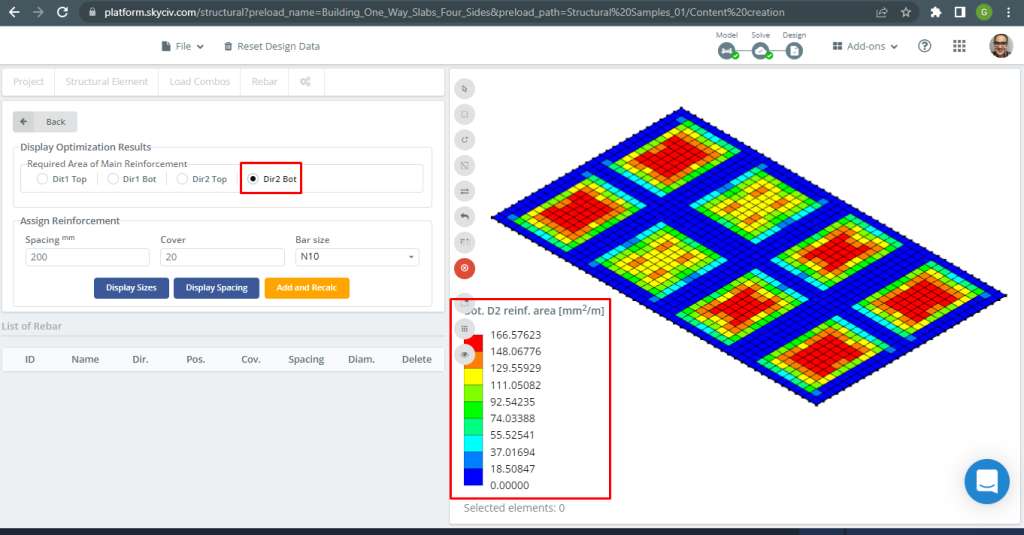
Figura 31. Refuerzo de barra de acero inferior en dirección 2. (SkyCiv Estructural 3D , Ingeniería en la nube SkyCiv).
Comparación de resultados
El último paso en este ejemplo de diseño de losa unidireccional es comparar el área de la barra de refuerzo de acero obtenida por análisis S3D y cálculos manuales..
Barra de acero para dirección X
| Momentos y área de acero | Negativo Exterior Izquierdo | Positivo Exterior | Negativo Exterior Derecho | Interior Negativo Izquierdo | Interior Positivo | Interior Negativo Derecha |
|---|---|---|---|---|---|---|
| \(UNA_{S t, Cálculos manuales} {milímetro^2}\) | 334.8214 | 334.8214 | 335.08233 | 334.821 | 334.8214 | 334.8214 |
| \(UNA_{S t, S3D} {milímetro^2}\) | 289.75 | 149.35 | 325.967 | 325.967 | 116.16 | 217.311 |
| \(\Delta_{diferencia}\) (%) | 13.461 | 55.39 | 2.720 | 2.644 | 65.307 | 35.0964 |
Barra de acero para dirección Y
| Momentos y área de acero | Negativo Exterior Izquierdo | Positivo Exterior | Negativo Exterior Derecho | Interior Negativo Izquierdo | Interior Positivo | Interior Negativo Derecha |
|---|---|---|---|---|---|---|
| \(UNA_{S t, Cálculos manuales} {milímetro^2}\) | 334.821 | 334.821 | 334.821 | 334.821 | 334.821 | 334.821 |
| \(UNA_{S t, S3D} {milímetro^2}\) | 270.524 | 156.75 | 304.34 | 304.34 | 156.75 | 270.52 |
| \(\Delta_{diferencia}\) (%) | 19.203 | 53.184 | 9.104 | 9.104 | 53.184 | 19.204 |
La diferencia es algo alta para los momentos positivos y la razón sería la presencia de vigas con alta rigidez torsional que impactan en los resultados del análisis de elementos finitos de la placa y los cálculos para la flexión del acero de refuerzo..
Si eres nuevo en SkyCiv, Regístrese y pruebe el software usted mismo!
Referencias
- Yew-Chaye Loo & Sanual Abrazo Chowdhury , “Hormigón armado y pretensado”, 2segunda edición, Prensa de la Universidad de Cambridge.
- Bazan Enrique & Meli Piralla, “Diseño Sísmico de Estructuras”, 1ed, CLARO.
- Estándar australiano, Estructuras de Hormigón, AS 3600:2018