
En diseño de conexión de acero, tornillos Generalmente se diseñan como un grupo de pernos que actúa como un solo cuerpo para resistir una carga determinada.. La resistencia de un grupo de pernos normalmente se establece mediante la resistencia de control de su perno más crítico.. Las cargas directas se distribuyen entre el número total de pernos, mientras que el momento inducido debido a la excentricidad de la carga se distribuye en relación con el momento de inercia del grupo de pernos y la distancia al centroide. Esto se llama análisis elástico.. Debido a sus supuestos simplificados y conservadores sobre la distribución de carga., a menudo produce conexiones atornilladas sobrediseñadas.
Cuando se habla de ingeniería de valor y diseños económicos, La mayoría de los fabricantes prefieren el enfoque inelástico.. Requiere menos pernos para la misma magnitud de carga.. Para hacer el enfoque inelástico, el centro instantáneo de rotación (ICOR) método usando iteraciones es la mejor manera.
En este artículo, Demostramos cómo calcular la fuerza de un conexión atornillada utilizando el método ICOR. Las reacciones por perno se calculan usando la ecuación (7-1) en la página 7-7 del Manual de la 15ª Edición del AISC. Luego se utiliza para comprobar si la ubicación supuesta del centro instantáneo del grupo de tornillos es correcta.. Finalmente, una vez que tengamos la ubicación correcta del IC, Calculamos el coeficiente C del grupo de tornillos para determinar su resistencia..
trabajado a mano, El método ICOR es un proceso largo., porque encontrar el centro instantáneo (CI) es prueba y error. Con un solucionador de computadora, el CI de un grupo de pernos se encuentra mediante iteraciones programadas.. El Solucionador de grupo SkyCiv Bolt utiliza un método de iteración rápida para determinar la ubicación del IC y el coeficiente del grupo de pernos en segundos. Es utilizado tanto por AISC como por AS. 4100 módulos de conexión.
El ejemplo resuelto a continuación es el mismo cálculo que realiza el solucionador., Se muestra una mano larga para que puedas seguir lo que está haciendo..
Obtener las propiedades del grupo de tornillos
Comencemos con un análisis simple de un grupo de cuatro pernos cargados con una carga de corte vertical excéntrica de 10 kips . La excentricidad de la carga a lo largo del eje x es 4 pulgadas a la derecha del grupo de tornillos. El ángulo desde la vertical es cero y la excentricidad a lo largo del eje y es cero..
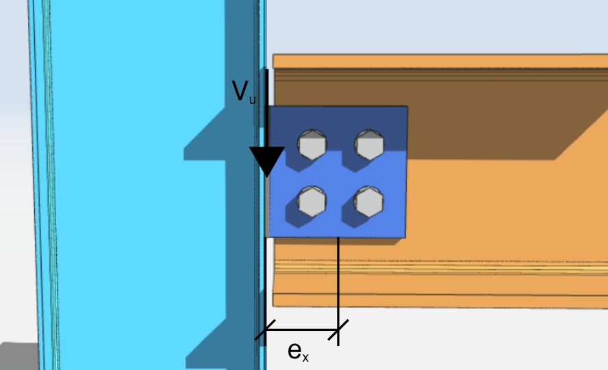
[math] V_{u} = 10\,kips [math]
[math] \theta = 0\,deg [math]
[math] e_{x} = 4\,in [math]
[math] e_{y} = 0\,in [math]
Lo primero que debe hacer es obtener las coordenadas de todos los tornillos del grupo.. Se recomiendan guías visuales y tablas..
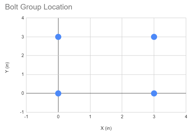
| Identificación de la tienda | X (in) | Y (in) |
| 1 | 0 | 0 |
| 2 | 0 | 3 |
| 3 | 3 | 0 |
| 4 | 3 | 3 |
Para obtener el centroide del grupo de tornillos a lo largo de los ejes x e y, necesitamos la siguiente fórmula.
Dejar [mathin] n [mathin] = número total de pernos
[math] X_{CG} = \frac{\sum X}{n} [math]
[math] Y_{CG} = \frac{\sum Y}{n} [math]
Luego, nuestra solución es:
[math] X_{CG} = \frac{\sum X}{n} = \frac{0\,in + 0\,in + 3\,in + 3\,in}{4} = 1.5\,in [math]
[math] Y_{CG} = \frac{\sum Y}{n} = \frac{0\,in + 3\,in + 0\,in + 3\,in}{4} = 1.5\,in [math]
Asumir la ubicación del I.C..
Después de obtener el centroide, asumimos la ubicación del centro instantáneo (CI). como primer intento, Podemos asumir que el IC se encuentra en el centroide geométrico del grupo de tornillos..
Entonces, asumir
[math] X_{IC} = X_{CG} = 1.5\,in [math]
[math] Y_{IC} = Y_{CG} = 1.5\,in [math]
Luego tabulamos el desplazamiento de cada perno del IC.. Obtenga primero la distancia a lo largo de x y la distancia a lo largo de y, entonces el desplazamiento resultante.
| Identificación de la tienda | cx (in) | cy (in) | c (in) |
| 1 | -1.5 | -1.5 | 2.121 |
| 2 | -1.5 | 1.5 | 2.121 |
| 3 | 1.5 | -1.5 | 2.121 |
| 4 | 1.5 | 1.5 | 2.121 |
Dónde,
[math] c_{x} = X_{i} – X_{IC} [math]
[math] c_{y} = Y_{i} – Y_{IC} [math]
[math] c = \sqrt{ {\left( c_{x} \right)}^{2} + {\left( c_{y} \right)}^{2} } [math]
Para perno No.. 1, nuestra solución es
[math] c_{x} = 0\,in – 1.5\,in = -1.5\,in [math]
[math] c_{y} = 0\,in – 1.5\,in = -1.5\,in [math]
[math] c = \sqrt{ {\left( -1.5\,in \right)}^{2} + {\left( -1.5\,in \right)}^{2} } = 2.121\,in [math]
Calcule la deformación por perno respecto a la distancia desde IC
Después de obtener las distancias de los pernos desde la ubicación supuesta del IC, calculamos la deformación de cada perno en función de su distancia.
La deformación máxima por perno., [mathin] \Delta_{max} = 0.34\,in [mathin], se basa en datos experimentales para un perno ASTM como se describe en la página AISC 7-8. Por proporción lineal, y configuración [mathin] \Delta_{max} = 0.34\,in [mathin], podemos calcular la deformación de un perno individual en relación con su participación en la distancia máxima [mathin] c_{max} [mathin]. La ecuación para obtener [mathin] \Delta [mathin] se muestra a continuación.
[math] \Delta_{1} = 0.34\,in \times \left( \frac{c}{c_{max}} \right) [math]
Para perno No.. 1, la deformación es
[math] \Delta_{1} = 0.34\,in \times \left( \frac{2.121\,in}{2.121\,in} \right) = 0.34\,in [math]
Porque el IC se asumió en el centroide, Los cuatro tornillos están a la misma distancia., para que los cuatro alcancen la misma deformación. Las deformaciones calculadas se tabulan a continuación..
| Identificación de la tienda | [mathin] \Delta [mathin] (in) |
| 1 | 0.34 |
| 2 | 0.34 |
| 3 | 0.34 |
| 4 | 0.34 |
Obtener las reacciones por perno
Una vez que tenemos la deformación por tornillo, Usamos AISC 15ª Ed.. Eq (7-1) para obtener las reacciones por tornillo.
[math] R = R_{ult} \left( 1 – e^{-10\Delta} \right)^{0.55} [math]
El [mathin] R_{ult} [mathin] en la ecuación es la carga última asumida sobre un perno, que podemos establecer como la resistencia a cortante del perno.
[math] R_{ult} = \phi R_{n} [math]
Para nuestro ejemplo, utilizamos una resistencia al corte del perno de [mathin] 24.4\,kip [mathin]. Otro valor es igualmente válido., porque se cancela cuando calculamos el coeficiente del grupo de tornillos [mathin] C [mathin] mas tarde.
Para perno No.. 1, la reacción calculada es
[math] R = R_{ult} \left( 1 – e^{-10\Delta} \right)^{0.55} [math]
[math] R = 24.4\,kip \left( 1 – e^{-10 \times \left( 0.34\,in \right)} \right)^{0.55} [math]
[math] R = 23.949\,kip [math]
Para el resto de los tornillos, las reacciones calculadas son las siguientes. Los componentes de la reacción del perno. [mathin] R [mathin] a lo largo de x e y también se muestran.
| Identificación de la tienda | R (kip) | Rx (kip) | Ry (kip) |
| 1 | 23.949 | 16.937 | -16.937 |
| 2 | 23.949 | -16.937 | -16.937 |
| 3 | 23.949 | 16.937 | 16.937 |
| 4 | 23.949 | -16.937 | 16.937 |
| ⅀Rx = 0 | ⅀ Ry = 0 |
La fuerza de cada perno actúa perpendicular a la línea que une ese perno al IC., que es lo que marca el signo de sus dos componentes. Para Perno No.1, Las soluciones para los componentes x e y se muestran a continuación..
[math] R_{x} = -R \left( \frac{c_{y}}{c} \right) = -23.949 \times \left( \frac{-1.5\,in}{2.121\,in} \right) = 16.937\,kip [math]
[math] R_{y} = R \left( \frac{c_{x}}{c} \right) = 23.949 \times \left( \frac{-1.5\,in}{2.121\,in} \right) = -16.937\,kip [math]
A continuación necesitamos el momento que produce cada reacción de perno sobre el IC.. Usa los componentes [mathin] R_{x} [mathin] y [mathin] R_{y} [mathin] con los brazos de palanca [mathin] c_{y} [mathin] y [mathin] c_{x} [mathin].
[math] M_{r} = -R_{x} c_{y} + R_{y} c_{x} [math]
Para Perno No.1, el momento en que la reacción sobre el IC es
[math] M_{r} = -16.937\,kip \times \left( -1.5\,in \right) + \left( -16.937\,kip \right) \times \left( -1.5\,in \right) [math]
[math] M_{r} = 50.811\,kip\text{-}in [math]
como cheque, el mismo momento es [mathin] R \times c = 23.949 \times 2.121 = 50.8\,kip\text{-}in [mathin], porque la fuerza es perpendicular al radio.
Cada perno aquí se encuentra a la misma distancia del IC asumido y lleva la misma fuerza., para que cada rayo regrese en el mismo momento. Las reacciones del momento se tabulan a continuación..
| Identificación de la tienda | Señor (pollo en) |
| 1 | 50.811 |
| 2 | 50.811 |
| 3 | 50.811 |
| 4 | 50.811 |
| ⅀señor = 203.244 |
Verificación de la ubicación del IC
Ahora que tenemos las reacciones de cortante y momento por tornillo, Los usamos para determinar la carga que resiste este grupo de pernos.. Tome la resultante de la suma de todas las reacciones a lo largo de x y la suma de todas las reacciones a lo largo de y.
De la sección anterior, calculamos que
[math] \sum R_{x} = 0\,kip [math]
y
[math] \sum R_{y} = 0\,kip [math]
Entonces,
[math] P_{u} = \sqrt{ {\left( \sum R_{x} \right)}^{2} + {\left( \sum R_{y} \right)}^{2} } = 0\,kip [math]
La carga resultante es [mathin] P_{u} = 0\,kip [mathin]. Un grupo de pernos que gira alrededor de su propio centroide conlleva un momento puro y ninguna fuerza neta., por lo que no puede resistir el corte aplicado. Eso ya nos dice que la primera ubicación asumida del IC es incorrecta, y podríamos parar aquí. Para el propósito de esta discusión, Continuaremos con los pasos restantes..
[math] P_{ux} = -P_{u}\sin\left( \theta \right) = 0\,kip [math]
[math] P_{uy} = -P_{u}\cos\left( \theta \right) = 0\,kip [math]
[math] M_{u} = -P_{ux}\left( Y_{CG} + e_{y} – Y_{IC} \right) + P_{uy} \left( X_{CG} + e_{x} – X_{IC} \right) = 0\,kip\text{-}in [math]
Ya que,
[math] P_{ux} \neq \sum R_{x} [math]
[math] P_{uy} \neq \sum R_{y} [math]
[math] M_{u} \neq \sum M_{r} [math]
El momento aplicado es cero mientras que las reacciones del perno suman 203.244 pollo en, entonces el equilibrio no se satisface. La supuesta ubicación del I.C.. Es incorrecto, y nos trasladamos a la siguiente ubicación supuesta.
SkyCiv tiene el cálculo del grupo de pernos integrado en sus módulos de diseño de conexiones. Quiere probar nuestro software de diseño de conexiones?
Segunda iteración
Para nuestra segunda iteración, supongamos que el I.C.. se encuentra en las coordenadas que se muestran a continuación. Porque la carga es un corte hacia abajo aplicado a la derecha del grupo., el verdadero IC se encuentra a la izquierda del centroide, entonces el juicio avanza en esa dirección.
Asumir
[math] X_{IC} = 0.062\,in [math]
[math] Y_{IC} = 1.5\,in [math]
Luego repita los pasos de la primera iteración.. La siguiente tabla muestra las coordenadas., la distancia de cada perno desde el I.C., y la deformación correspondiente con respecto a esa distancia.
| Identificación de la tienda | X (in) | Y (in) | cx (in) | cy (in) | c (in) | [mathin] \Delta [mathin] (in) |
| 1 | 0 | 0 | -0.062 | -1.5 | 1.501 | 0.155 |
| 2 | 0 | 3 | -0.062 | 1.5 | 1.501 | 0.155 |
| 3 | 3 | 0 | 2.938 | -1.5 | 3.299 | 0.34 |
| 4 | 3 | 3 | 2.938 | 1.5 | 3.299 | 0.34 |
Esta vez los pernos no están todos a la misma distancia del IC., entonces solo el par lejano llega al 0.34 en limite. El par cercano se deforma menos y por tanto soporta menos carga..
Tenga en cuenta que el centroide calculado de la grupo de pernos no ha cambiado, ya que las coordenadas del perno no se han movido.
[math] X_{CG} = 1.5\,in [math]
[math] Y_{CG} = 1.5\,in [math]
Luego calculamos las reacciones a lo largo de x, las reacciones a lo largo de y, y el momento correspondiente. Los valores se tabulan a continuación..
| Identificación de la tienda | R (kip) | Rx (kip) | Ry (kip) | Señor (pollo en) |
| 1 | 21.4 | 21.4 | -0.9 | 32.1 |
| 2 | 21.4 | -21.4 | -0.9 | 32.1 |
| 3 | 23.9 | 10.9 | 21.3 | 79.0 |
| 4 | 23.9 | -10.9 | 21.3 | 79.0 |
| ⅀Rx = 0 | ⅀ Ry = 41 | ⅀señor = 222 |
próximo, determinamos la carga resultante de todas las reacciones a lo largo de x e y.
[math] P_{u} = \sqrt{ {\left( \sum R_{x} \right)}^{2} + {\left( \sum R_{y} \right)}^{2} } [math]
[math] P_{u} = \sqrt{ {\left( 0\,kip \right)}^{2} + {\left( 40.703\,kip \right)}^{2} } [math]
[math] P_{u} = 40.703\,kip [math]
Entonces los componentes de la carga resultante, basado en lo dado [mathin] \theta [mathin], se muestran a continuación.
[math] P_{ux} = -P_{u}\sin\left( \theta \right) = -41\,kip \times \sin\left( 0\,deg \right) = 0\,kip [math]
[math] P_{uy} = -P_{u}\cos\left( \theta \right) = -41\,kip \times \cos\left( 0\,deg \right) = -41\,kip [math]
Luego usamos estos componentes para resolver la carga de momento alrededor del I.C asumido..
[math] M_{u} = -P_{ux} \left( Y_{CG} + e_{y} – Y_{IC} \right) + P_{uy} \left( X_{CG} + e_{x} – X_{IC} \right) [math]
[math] M_{u} = -0\,kip \left( 1.5\,in + 0\,in – 1.5\,in \right) + \left( -41\,kip \right) \left( 1.5\,in + 4\,in – 0.062\,in \right) [math]
[math] M_{u} = -222\,kip\text{-}in [math]
próximo, comparemos el calculado [mathin] P_{ux} [mathin], [mathin] P_{uy} [mathin] y [mathin] M_{u} [mathin] contra las reacciones del grupo de tornillos.
[math] P_{ux} \approx -\sum R_{x} [math]
[math] P_{uy} \approx -\sum R_{y} [math]
[math] M_{u} \approx -\sum M_{r} [math]
Numéricamente eso es 0 contra 0, -41 saltar contra -41 kip, y -222 entrar en contra -222 pollo en. El lado izquierdo está lo suficientemente cerca del lado derecho como para que podamos tomar la ubicación supuesta del I.C.. como correcto.
En la práctica, el solucionador sigue moviendo el CI de prueba hasta que estos tres residuos caen dentro de una tolerancia., en lugar de detenerse en una coincidencia visual.
Resolviendo para el coeficiente C
Una vez que el I.C.. la ubicación está determinada, Podemos obtener el coeficiente C del grupo de tornillos con la siguiente fórmula..
[math] C = \frac{P_{u}}{\phi R_{n}} = \frac{40.703\,kip}{24.4\,kip} = 1.668 [math]
El coeficiente significa que el grupo lleva 1.668 veces la fuerza de un solo perno. Tenga en cuenta que esto está muy por debajo de los cuatro tornillos presentes., porque la excentricidad le cuesta al grupo la mayor parte de su capacidad nominal. Es también donde la elección de [mathin] R_{ult} [mathin] cancela, es por eso que cualquier valor consistente podría usarse al principio.
Calculadora de grupo de tornillos libres
Vea cómo diseñamos nuestras conexiones atornilladas con este enfoque en el módulo de diseño de conexiones.. Elija una conexión atornillada, establecer la disposición del perno y la excentricidad, y el informe proporciona la ubicación del IC y el coeficiente C junto con todas las demás comprobaciones.. Se ejecuta en el navegador., sin nada que instalar.
Para más funcionalidad, incluyendo guardar y recargar sus archivos, regístrate para obtener una cuenta gratuita.
