Vloersystemen die door de norm worden beschouwd
Australische normen stellen de minimumvereisten vast voor het ontwerp van platen van gewapend beton, zoals eenrichtings- en tweerichtingstypen. Wat betreft de plattegrondconfiguratie en het opnemen van liggers, de platen kunnen ook worden verdeeld in vierzijdig ondersteunde platen, balk-en-plaat systemen, vlakke platen, en vlakke platen. Deze typen zijn samengevat in de volgende afbeeldingen.
Vereenvoudig de naleving van het Australische plaatontwerp met de geavanceerde SkyCiv concreet-rapport-voorbeeld. Probeer het eens! AS eenvoudig aanbrengen 3600 controles op platen en vlakke platen.
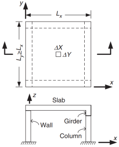
Figuur 1. Aan vier zijden ondersteunde plaat. (Yew-Chaye Loo & Sanual knuffel Chowdhury , “Gewapend en voorgespannen beton”, 2e editie, Cambridge University Press).
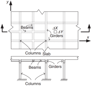
Figuur 2. Grillage Slab-systeem. (Yew-Chaye Loo & Sanual knuffel Chowdhury , “Gewapend en voorgespannen beton”, 2e editie, Cambridge University Press).
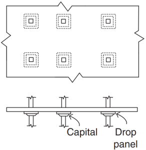
Figuur 3. Platte platen. (Yew-Chaye Loo & Sanual knuffel Chowdhury , “Gewapend en voorgespannen beton”, 2e editie, Cambridge University Press).
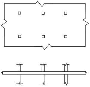
Figuur 4. Platte Platen. (Yew-Chaye Loo & Sanual knuffel Chowdhury , “Gewapend en voorgespannen beton”, 2e editie, Cambridge University Press).
De Standaard beveelt enkele methodes aan (vereenvoudigde en beproefde procedures) bij het bepalen van buigmomenten:
- Clausule 6.10.2: Doorlopende liggers en eenrichtingsplaten
- Clausule 6.10.3: Aan vier zijden ondersteunde tweerichtingsplaten
- Clausule 6.10.4: Tweerichtingsplaten met meerdere overspanningen
Het doel van de code is om de totale hoeveelheid wapeningsstaal te ontwerpen in hoofdrichtingen in het plaatsysteem. Voor de buigmomenten wordt wapeningsstaal berekend “Mx” en “Mijn.” Figuur 5 toont de andere krachten of acties in een eindig plaatelement waarin de code hun weerstandswaarden voorschrijft.
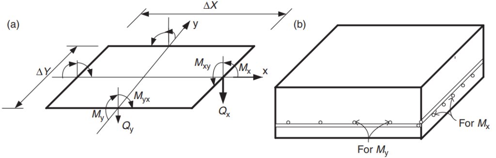
Figuur 5. Krachten in een eindig plaatelement: buigende momenten (Mx, Mijn), draaiende momenten (Mxy, Myx), en scharen (Qx, Qy). (Yew-Chaye Loo & Sanual knuffel Chowdhury , “Gewapend en voorgespannen beton”, 2e editie, Cambridge University Press)
In dit artikel, we zullen twee plaatontwerpvoorbeelden ontwikkelen, eenrichtings- en tweerichtingsplaatsystemen, met behulp van de vereenvoudigde methoden die door de code zijn georiënteerd en toegestaan. In beide gevallen, we zullen een SkyCiv S3D-model maken en de resultaten vergelijken met de hierboven genoemde methoden.
Als je nieuw bent bij SkyCiv, Meld u aan en test de software zelf!
Ontwerpvoorbeeld van eenrichtingsplaat
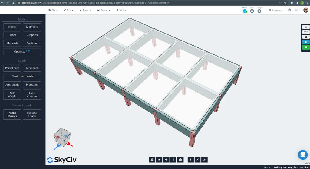
Hieronder ziet u het kleine gebouw en de platen die we zullen ontwerpen
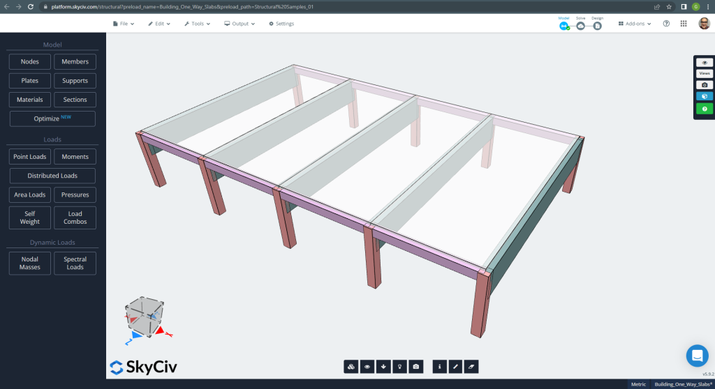
Figuur 6. Eenrichtingsplaten in een klein bouwvoorbeeld. (Structurele 3D, SkyCiv Cloud-engineering).
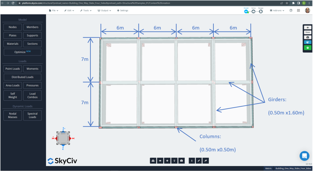
De planafmetingen worden hieronder weergegeven
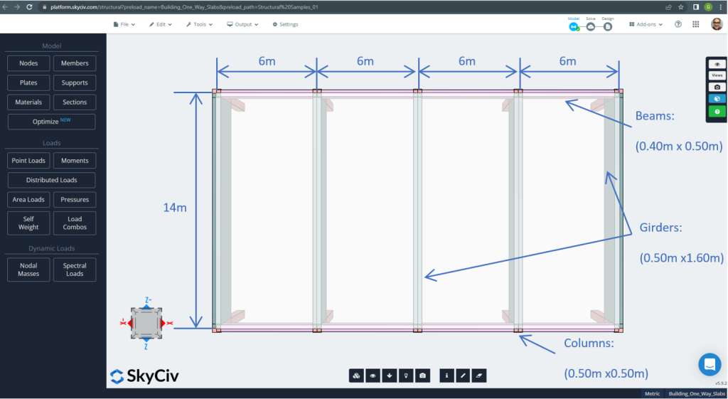
Figuur 7. Planafmetingen en structurele elementen. (Structurele 3D, SkyCiv Cloud-engineering).
Voor het plaatvoorbeeld, samengevat, het materiaal, elementen eigenschappen, en veel om over na te denken :
- Classificatie van plaattypes: Een – manier gedrag \(\frac{L_2}{L_1} > 2 ; \frac{14m}{6m}=2,33 > 2.00 \) OK!
- Bezetting gebouw: Residentieel gebruik
- Plaatdikte \(t_{plaat}=0,25m)
- Gewapend betondichtheid uitgaande van een staalwapeningsverhouding van 0.5% \(\rho_w = 24 \frac{kN}{m^3} + 0.6 \frac{kN}{m^3} \keer 0.5 = 24.3 \frac{kN}{m^3} \)
- Beton karakteristieke druksterkte bij 28 dagen \(f'c = 25 MPa \)
- Betonelasticiteitsmodulus volgens Australian Standard \(E_c = 26700 MPa \)
- Eigen gewicht van plaat \(Dead = \rho_w \times t_{plaat} = 24.3 \frac{kN}{m^3} \maal 0,25m= 6.075 \frac {kN}{m^2}\)
- Superopgelegde eigen last \(SD = 3.0 \frac {kN}{m^2}\)
- Live laden \(L = 2.0 \frac {kN}{m^2}\)
Handmatige berekening volgens AS3600-standaard
In deze sectie, we berekenen de vereiste gewapende stalen wapening met behulp van de referentie van de Australische norm. We verkrijgen eerst het totale meegerekende buigmoment dat moet worden uitgevoerd door de strook met eenheidsbreedte van de plaat.
- Dode lading, \(g = (3.0 + 6.075) \frac{kN}{m^2} \keer 1 m = 9.075 \frac{kN}{m}\)
- Live laden, \(q = (2.0) \frac{kN}{m^2} \keer 1 m = 2.0 \frac{kN}{m}\)
- Ultieme lading, \(Fd = 1.2\times g + 1.5\keer q = (1.2\keer 9.075 + 1.5\keer 2.0)\frac{kN}{m} =13.89 \frac{kN}{m} \)
Gebruikmakend van de vereenvoudigde methode gespecificeerd door de standaard, eerste, het is een must om aan de volgende beperkingen te voldoen:
- \(\frac{L_i}{L_j} \de 1.2 . \frac{6m}{6m} Hieronder volgen de verschillende manieren om de gronddrukcoëfficiënten te bepalen om de eenheidswrijvingsweerstand van palen in zand te berekenen < 1.2 \). OK!
- De belasting moet uniform zijn. OK!
- \(q \le 2g. q=2 \frac{kN}{m} < 18.15 \frac{kN}{m}\). OK!
- De dwarsdoorsnede van de plaat moet uniform zijn. OK!.
Aanbevolen minimale dikte, d
\(d \ge \frac{L_{bijv}}{{k_3}{k_4}{\sqrt[3]{\frac{\frac{\Delta}{L_{ef}}{E_c}}{F_{d, ef}}}}}\)
Waarbij
- \(k_3 = 1.0; k_4 = 1.75 \)
- \(\frac{\Delta}{L_{ef}}=1/250 \)
- \(E_c = 27600 MPa \)
- \(F_{d,ef} = (1.0 +zodat ingenieurs precies kunnen nagaan hoe deze berekeningen zijn gemaakt{cs})\maal g + (\psi_s + zodat ingenieurs precies kunnen nagaan hoe deze berekeningen zijn gemaakt{cs}\times \psi_1) \maal q=(1.0+0.8)\keer 9.075 + (0.7+0.8\keer 0.4)\keer 2 = 18.375 kPa\)
- \(\psi_s = 0.7 \) Live-load kortetermijnfactor
- \(\psi_1 = 0.4 \) Levensduurfactor op lange termijn
- \(zodat ingenieurs precies kunnen nagaan hoe deze berekeningen zijn gemaakt{cs} = 0.8 \)
\(d \ge \frac{5.50m}{{1.0}\keer {1.75}{\sqrt[3]{\frac{\frac{1}{250}\keer{27600 \maal 10^3 kPa}}{18.375 kPa}}}} \ge 0,173m. d = 0,25 m > 0.173m \) OK!
Zodra we hebben aangetoond dat aan de beperkingen is voldaan, het buigmoment wordt berekend met behulp van de uitdrukking: \(M=\alpha \times F_d \times L_n^2\) waar \(\alfa) is een constante gedefinieerd in de volgende afbeelding.
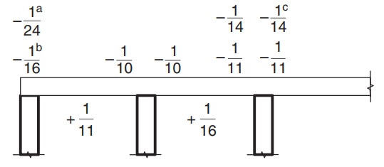
Figuur 8. Waarden van momentcoëfficiënt \(\alfa) voor platen met meer dan twee overspanningen. (Yew-Chaye Loo & Sanual knuffel Chowdhury , “Gewapend en voorgespannen beton”, 2e editie, Cambridge University Press).
Waarbij:
- (een) Geval van platen en balken op steunbalken
- (b) Alleen voor doorlopende balkondersteuning
- (c) Waar klasse L-wapening wordt gebruikt
- \(L_n \) is de eenheidsstrookoverspanning
- \(F_d \) is de zwaartekrachtfactored belasting
Voor het plaatvoorbeeld, we moeten case gebruiken (een) omdat de plaat op stijve liggers rust. Er zal slechts één geval worden uitgelegd en de rest zal in de volgende tabel worden weergegeven. We nemen ook de berekening van het staalwapeningsoppervlak mee.
- \(M={\alfa} {F_d}{L_n^2}={-\frac{1}{24}}\keer {13.89 \frac{kN}{m}}\keer (6m-0.5m)➔⡔ Koop generieke tadalafil – 17.51{kN}{m}\)
- Afdekking = 20 mm (Een minimum van 10 mm is nodig voor een brandwerendheidsperiode van 60 minuten).
- \(d = t_{plaat} – Hoes – \frac{BarDiameter}{2} = 250 mm – 20mm – 6mm = 224 mm \)
- \(\alpha_2 = 1.0-0.003 f’c = 1.0-0.003\times 25 = 0.925 (0.67 \le \alpha_2 \le 0.85) \) Dus, wij selecteren \(\alpha_2 = 0.85\)
- \(\xi = \frac{\alpha_2\times f’c}{f_{de opwaartse bodemdruk veroorzaakt bidirectionele buiging met trekspanningen aan het bodemoppervlak}} = frac{0.85\keer 25 MPa}{500 MPa} = 0.0425 \)
- \(\rho_t = \xi – \sqrt{{\xi}^ 2 – \frac{{2}{\xi}{M}}{{\phi}{b}{d^2}{f_{de opwaartse bodemdruk veroorzaakt bidirectionele buiging met trekspanningen aan het bodemoppervlak}}}} = 0.0425 – \sqrt{{0.0425}^2-\frac{2\times 0.0425\times 17.51{kN}{m}}{{0.8}\keer {1m}\keer {{(0.224m)^ 2}} \keer {500\keer {10^3}kPa}}}=0.0008814\)
- \(\gamma= 1.05-0.007 f’c = 1.05-0.007\times 25 = 0.875 (0.67 \le \gamma \le 0.85) \) Dus, wij selecteren \(\gamma = 0.85\)
- \(k_u = \frac{\rho_t \times f_{de opwaartse bodemdruk veroorzaakt bidirectionele buiging met trekspanningen aan het bodemoppervlak}}{0.85\times \gamma \times f’c}= frac{0.0008814\keer 500 MPa}{0.85\keer 0.85 \keer 25 MPa} =0.0244\)
- \(\phi = 1.19 – \frac{13\zodat ingenieurs precies kunnen nagaan hoe deze berekeningen zijn gemaakt{u0}}{12} = 1.19 – \frac{13\keer 0.0244}{12} = 1.164 (0.6 \le \phi \le 0.8) \) Dus, wij selecteren \(\phi = 0.8\). OK!.
- \(\de opwaartse bodemdruk veroorzaakt bidirectionele buiging met trekspanningen aan het bodemoppervlak{t,min} = 0.20 {(\frac{D}{d})^ 2}{(\frac{f'_{ct,f}}{f_{de opwaartse bodemdruk veroorzaakt bidirectionele buiging met trekspanningen aan het bodemoppervlak}})} = 0.20 \keer (\frac{0.25m}{0.224m})^2 \times \frac{0.6\keer sqrt{25MPa}}{500 MPa} = 0.0015\)
- \(EEN_{de opwaartse bodemdruk veroorzaakt bidirectionele buiging met trekspanningen aan het bodemoppervlak}=max(\de opwaartse bodemdruk veroorzaakt bidirectionele buiging met trekspanningen aan het bodemoppervlak{t,min}, \rho_t)\times b \times d = max(0.0015,0.0008814)\keer 1000 mm \times 224 mm= 334.82 mm^2 \)
| \(\alfa) en Momenten | Exterieur Negatief Links | Exterieur Positief | Exterieur negatief recht | Binnenlands Negatief Links | Interieur Positief | Binnenlands negatief recht |
|---|---|---|---|---|---|---|
| \(\alfa) toe te passen | -\(\frac{1}{24}\) | \(\frac{1}{11}\) | -\(\frac{1}{10}\) | \(\frac{1}{10}\) | \(\frac{1}{16}\) | \(\frac{1}{11}\) |
| M-waarde | -17.51 | 38.20 | -42.02 | 42.02 | 26.26 | 38.20 |
| \(\rho_t\) | 0.0008814 | 0.001948 | 0.002148 | 0.002148 | 0.00133 | 0.001948 |
| naar | 0.0244 | 0.0539 | 0.0594 | 0.0594 | 0.0368 | 0.05391 |
| \(\phi) | 0.8 | 0.8 | 0.8 | 0.8 | 0.8 | 0.8 |
| \(EEN_{de opwaartse bodemdruk veroorzaakt bidirectionele buiging met trekspanningen aan het bodemoppervlak} {mm^2}\) | 334.82 | 436.31 | 481.099 | 481.099 | 334.8214 | 436.3100 |
Na de berekening van het wapeningsoppervlak, je kunt de detaillering definiëren (de daadwerkelijke manier om de wapening in de plaat te plaatsen). Als hulp voor uw weten, wij delen het volgende beeld, die de wapeningslocatie voor positieve en negatieve momenten aangeeft:
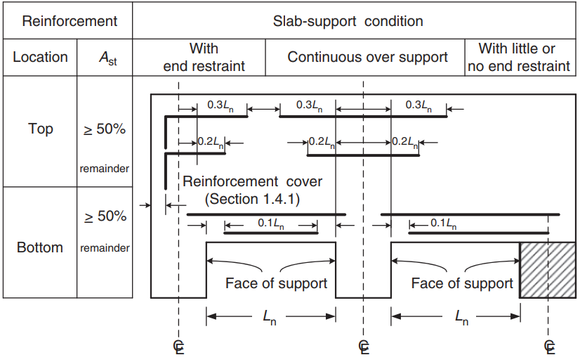
Figuur 9. Versterkingsarrangement voor één- en tweerichtingsplaten. (Yew-Chaye Loo & Sanual knuffel Chowdhury , “Gewapend en voorgespannen beton”, 2e editie, Cambridge University Press)
Als je nieuw bent bij SkyCiv, Meld u aan en test de software zelf!
Resultaten van de SkyCiv S3D-plaatontwerpmodule
In de eerste weergave, we zullen enkele afbeeldingen tonen voor de modellering en structurele analyse van het voorbeeld in S3D. We raden u aan om via de volgende links meer te lezen over modelleren in SkyCiv Hoe platen te modelleren? Elke keer dat je een nieuwe toevoegt ACI-plaatontwerpvoorbeeld met SkyCiv.
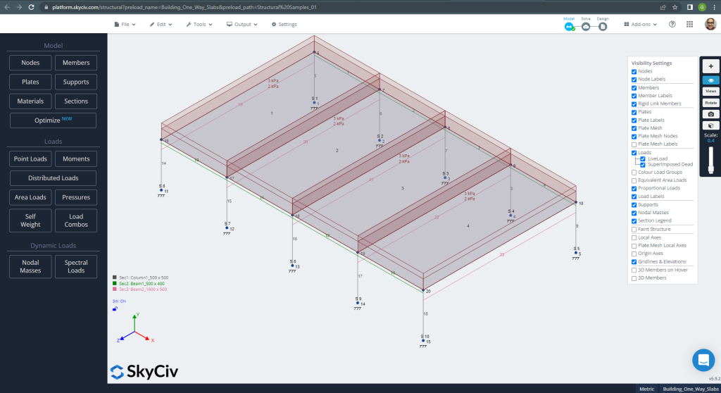
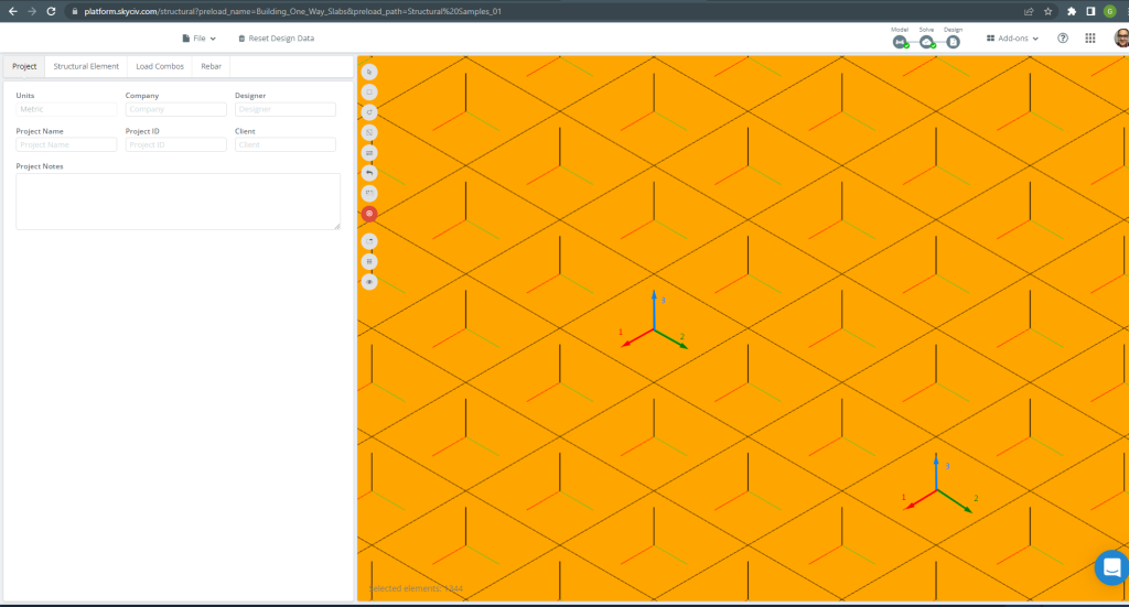
Figuur 10. Structureel model in S3D voor eenrichtingsplaten voorbeeld. (Structurele 3D, SkyCiv Cloud-engineering).
Voordat u het model analyseert, we moeten een plaatmaaswijdte definiëren. Enkele referenties (2) adviseer een maat voor het schaalelement van 1/6 van de korte overspanning of 1/8 van de lange spanwijdte, hoe korter. Deze waarde volgen, wij hebben \(\frac{L2}{6}= frac{6m}{6} = 1 meter \) of \(\frac{L1}{8}= frac{14m}{8}=1,75m \); wij nemen 1m als maximale aanbevolen maat en 0,50m toegepaste maaswijdte.
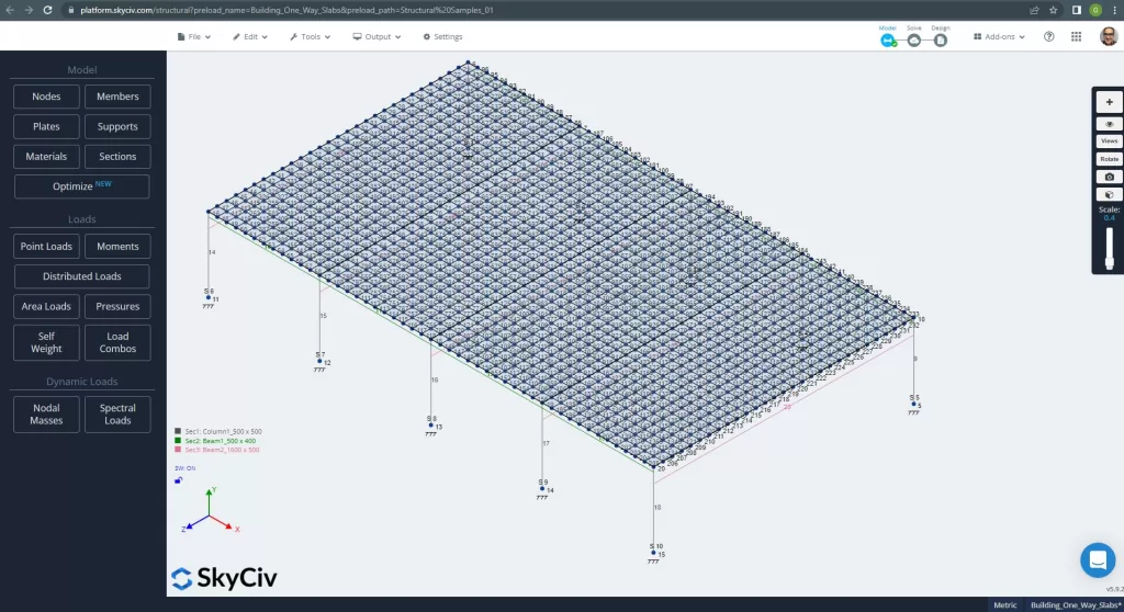
Figuur 11. Verbeterd gaas in platen. (Structurele 3D, SkyCiv Cloud-engineering).
Ooit hebben we ons analytisch structureel model verbeterd, we voeren een lineair-elastische analyse uit. Bij het ontwerpen van platen, we moeten controleren of de verticale verplaatsing kleiner is dan het maximum toegestaan door de code. Australian Standars heeft een maximale verticale verplaatsing van \(\frac{L}{250}= frac{6000mm}{250}=24.0 mm\).
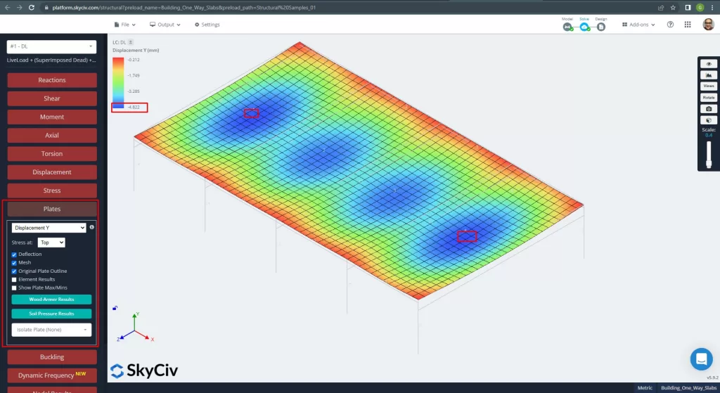
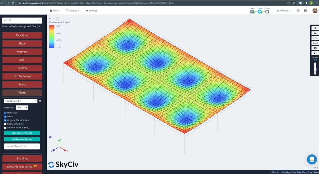
Figuur 12. Verticale verplaatsing in platen. (Structurele 3D, SkyCiv Cloud-engineering).
Vergelijking van de maximale verticale verplaatsing met de code waarnaar wordt verwezen, de stijfheid van de plaat is voldoende. \(4.822 mm < 24.00mm\).
De maximale momenten in de overspanningen van de plaat bevinden zich voor positief in het midden en voor negatief aan de buiten- en binnensteunen. Laten we deze momentenwaarden bekijken in de volgende afbeeldingen.
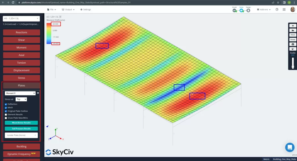
Figuur 13. Momenten in de X-richting. (Structurele 3D, SkyCiv Cloud-engineering).
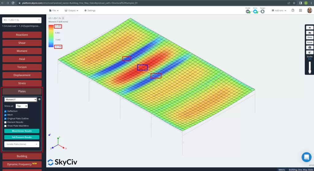
Figuur 14. Momenten in de Y-richting. (Structurele 3D, SkyCiv Cloud-engineering).
De lokale assen van plaatelementen worden hieronder aangegeven.
Figuur 15. Plaats lokale assen. (Structurele 3D, SkyCiv Cloud-engineering).
Voor meer details over het geautomatiseerd ontwerp van gewapende platen, zie onze documentatie Platen in SkyCiv.
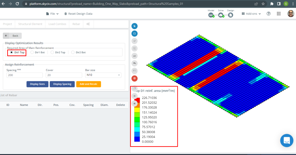
Figuur 16. Bovenste D1-versterking. (Structurele 3D, SkyCiv Cloud-engineering).
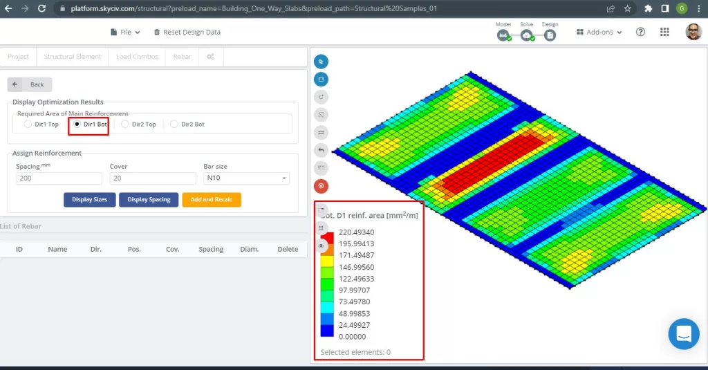
Figuur 17. Onderste D1-versterking. (Structurele 3D, SkyCiv Cloud-engineering).
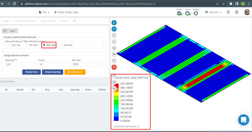
Figuur 18. Bovenste D2-versterking. (Structurele 3D, SkyCiv Cloud-engineering).
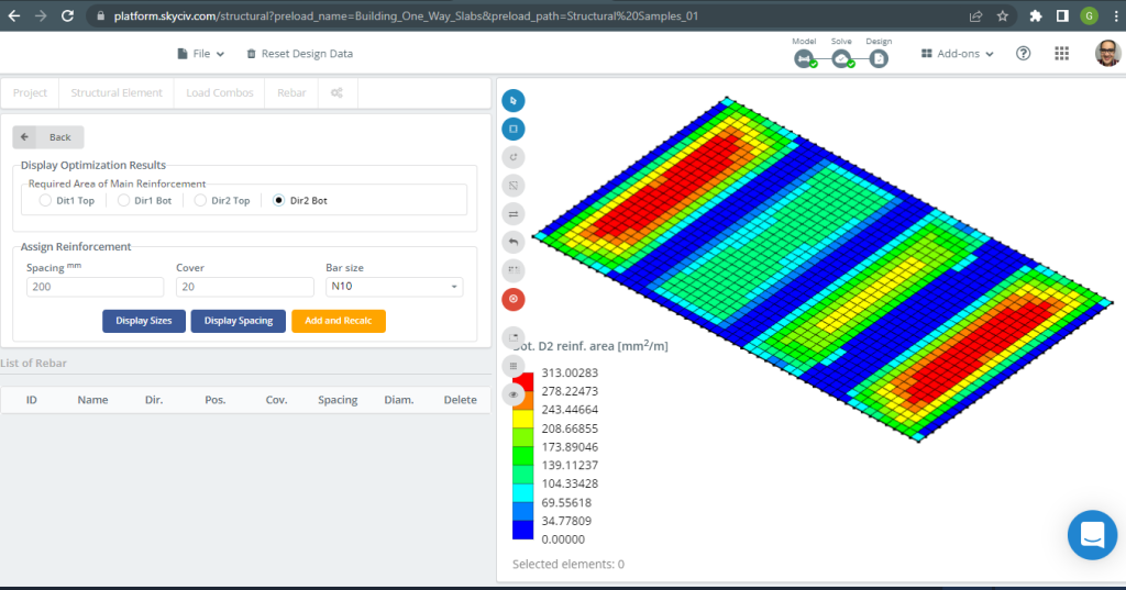
Figuur 19. Onderste D2-versterking. (Structurele 3D, SkyCiv Cloud-engineering).
Vergelijking van resultaten
De laatste stap in dit ontwerpvoorbeeld van een eenrichtingsplaat is het vergelijken van het gebied van de stalen wapening verkregen door S3D-analyse (lokale assen “2”) en handberekeningen.
| Momenten en staalgebied | Exterieur Negatief Links | Exterieur Positief | Exterieur negatief recht | Binnenlands Negatief Links | Interieur Positief | Binnenlands negatief recht |
|---|---|---|---|---|---|---|
| \(EEN_{de opwaartse bodemdruk veroorzaakt bidirectionele buiging met trekspanningen aan het bodemoppervlak, HandCalcs} {mm^2}\) | 334.82 | 436.31 | 481.099 | 481.099 | 334.8214 | 436.3100 |
| \(EEN_{de opwaartse bodemdruk veroorzaakt bidirectionele buiging met trekspanningen aan het bodemoppervlak, S3D} {mm^2}\) | 285.13 | 313.00 | 427.69 | 427.69 | 313.00 | 427.69 |
| \(\Delta_{verschil}\) (%) | 14.84 | 28.262 | 11.101 | 11.101 | 6.517 | 1.986 |
We kunnen zien dat de resultaten van de waarden zeer dicht bij elkaar liggen. Dit betekent dat de berekeningen correct zijn!
Ontwerpvoorbeeld van tweerichtingsplaten
In deze sectie, we zullen een voorbeeld ontwikkelen dat bestaat uit een grillagesysteem.
Figuur 20. Grillage-systeem. (Structurele 3D, SkyCiv Cloud-engineering).
De planafmetingen worden hieronder weergegeven
Figuur 21. Planafmetingen voor het voorbeeld van een tweezijdige plaat met vier zijden. (Structurele 3D, SkyCiv Cloud-engineering).
Voor het plaatvoorbeeld, samengevat, het materiaal, elementen eigenschappen, en veel om over na te denken :
- Classificatie van plaattypes: Twee – manier gedrag \(\frac{L_2}{L_1} \de 2 ; \frac{7m}{6m}=1,167 < 2.00 \) OK!
- Bezetting gebouw: Residentieel gebruik
- Plaatdikte \(t_{plaat}=0,25m)
- Gewapend betondichtheid uitgaande van een staalwapeningsverhouding van 0.5% \(\rho_w = 24 \frac{kN}{m^3} + 0.6 \frac{kN}{m^3} \keer 0.5 = 24.3 \frac{kN}{m^3} \)
- Beton karakteristieke druksterkte bij 28 dagen \(f'c = 25 MPa \)
- Betonelasticiteitsmodulus volgens Australian Standard \(E_c = 26700 MPa \)
- Eigen gewicht van plaat \(Dead = \rho_w \times t_{plaat} = 24.3 \frac{kN}{m^3} \maal 0,25m= 6.075 \frac {kN}{m^2}\)
- Superopgelegde eigen last \(SD = 3.0 \frac {kN}{m^2}\)
- Live laden \(L = 2.0 \frac {kN}{m^2}\)
Handmatige berekening volgens AS3600-standaard
In deze sectie, we berekenen de vereiste gewapende stalen wapening met behulp van de referentie van de Australische norm. We verkrijgen eerst het totale meegerekende buigmoment dat moet worden uitgevoerd door de stroken met eenheidsbreedte van de plaat in elke buighoofdrichting.
- Dode lading, \(g = (3.0 + 6.075) \frac{kN}{m^2} \keer 1 m = 9.075 \frac{kN}{m}\)
- Live laden, \(q = (2.0) \frac{kN}{m^2} \keer 1 m = 2.0 \frac{kN}{m}\)
- Ultieme lading, \(Fd = 1.2\times g + 1.5\keer q = (1.2\keer 9.075 + 1.5\keer 2.0)\frac{kN}{m} =13.89 \frac{kN}{m} \)
Ontwerpmomenten en coëfficiënten
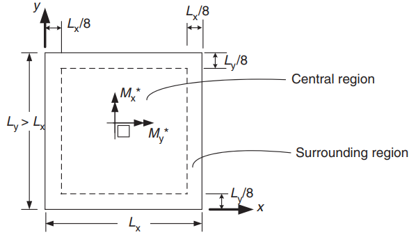
Figuur 22. Oriëntatie van een tweerichtingsplaat voor bepaling van positieve momenten. (Yew-Chaye Loo & Sanual knuffel Chowdhury , “Gewapend en voorgespannen beton”, 2e editie, Cambridge University Press)
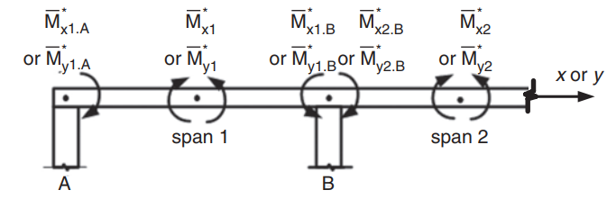
Figuur 23. Bepaling van negatieve momenten in een tweewegplaat. (Yew-Chaye Loo & Sanual knuffel Chowdhury , “Gewapend en voorgespannen beton”, 2e editie, Cambridge University Press)
| Randconditie | Coëfficiënten voor korte overspanningen (\(\beta_x\)) | Coëfficiënten over lange overspanningen (\(\beta_y)\) alle waarden van \(\frac{L_y}{L_x}\) | |||||||
|---|---|---|---|---|---|---|---|---|---|
| Waarden van \(\frac{L_y}{L_x}\) | |||||||||
| 1.0 | 1.1 | 1.2 | 1.3 | 1.4 | 1.5 | 1.75 | \(\geven 2.0\) | ||
| 1. Vier randen doorlopend | 0.024 | 0.028 | 0.032 | 0.035 | 0.037 | 0.040 | 0.044 | 0.048 | 0.024 |
| 2. Eén korte randdiscontinuos | 0.028 | 0.032 | 0.036 | 0.038 | 0.041 | 0.043 | 0.047 | 0.050 | 0.028 |
| 3. Eén lange rand is onderbroken | 0.028 | 0.035 | 0.041 | 0.046 | 0.050 | 0.054 | 0.061 | 0.066 | 0.028 |
| 4. Twee korte randen onderbroken | 0.034 | 0.038 | 0.040 | 0.043 | 0.045 | 0.047 | 0.050 | 0.053 | 0.034 |
| 5. Twee lange randen onderbroken | 0.034 | 0.046 | 0.056 | 0.065 | 0.072 | 0.078 | 0.091 | 0.100 | 0.034 |
| 6. Twee aangrenzende randen zijn onderbroken | 0.035 | 0.041 | 0.046 | 0.051 | 0.055 | 0.058 | 0.065 | 0.070 | 0.035 |
| 7. Drie randen onderbroken (één lange zijde doorlopend) | 0.043 | 0.049 | 0.053 | 0.057 | 0.061 | 0.064 | 0.069 | 0.074 | 0.043 |
| 8. Drie randen onderbroken (één korte zijde doorlopend) | 0.043 | 0.054 | 0.064 | 0.072 | 0.078 | 0.084 | 0.096 | 0.105 | 0.043 |
| 9. Vier randen discontinuo's | 0.056 | 0.066 | 0.074 | 0.081 | 0.087 | 0.093 | 0.103 | 0.111 | 0.056 |
Tafel 1. (Yew-Chaye Loo & Sanual knuffel Chowdhury , “Gewapend en voorgespannen beton”, 2e editie, Cambridge University Press)
In de volgende afbeelding worden alle negen gevallen uitgelegd waarnaar de bovenstaande tabel verwijst
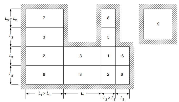
Figuur 24. Randvoorwaarden voor tweezijdige platen die aan vier zijden worden ondersteund. (Yew-Chaye Loo & Sanual knuffel Chowdhury , “Gewapend en voorgespannen beton”, 2e editie, Cambridge University Press)
Ontwerpmomenten voor centrale regio (Geval 6 Twee aangrenzende randen onderbroken) :
- \(L_x = 6m, L_y=7m, \frac{L_y}{L_x} = frac{7m}{6m}= 1.167 \) Waarden die lineair moeten worden geïnterpoleerd
- Positieven:
- \(M_x = {\beta_x}{F_d}{L_x^2} = {0.04435}\keer {13.89 \frac{kN}{m}}\keer{(6m)^ 2}=22.177 kNm\)
- \(Mijn_j = {\beta_y}{F_d}{L_x^2} ={0.035}\keer {13.89 \frac{kN}{m}}\keer{(6m)^ 2}=17,501 kNm \)
- Negatieven buitenoverspanning:
- \(M_{x1, EEN} = -\lambda_e \times M_x = -0.5 \keer 22.177 kNm = – 11.089 kNm\)
- \(M_{y1,A} = -\lambda_e \times M_y = -0.5 \keer 17.501 kNm = -8.751 kNm \)
- Negatieven binnenoverspanning:
- \(M_{x1, B} = -\lambda_{1X} \keer M_x = -1.33 \keer 22.177 kNm = – 29.495 kNm\)
- \(M_{j1, B} = -\lambda_{1j} \keer M_y = -1.33 \keer 17.501 kNm = -23.276 kNm \)
Ontwerpmomenten voor centrale regio (Geval 3 Eén lange rand is onderbroken) :
- \(L_x = 6m, L_y=7m, \frac{L_y}{L_x} = frac{7m}{6m}= 1.167 \) Waarden die lineair moeten worden geïnterpoleerd
- Positieven:
- \(M_x = {\beta_x}{F_d}{L_x^2} = {0.03902}\keer {13.89 \frac{kN}{m}}\keer{(6m)^ 2}= 19.512 kNm\)
- \(Mijn_j = {\beta_y}{F_d}{L_x^2} ={0.028}\keer {13.89 \frac{kN}{m}}\keer{(6m)^ 2}= 14.001 kNm \)
- Negatieven binnenoverspanning:
- \(M_{x1, B} = -\lambda_{1X} \keer M_x = -1.33 \keer 19.512 kNm = – 25.951 kNm\)
- \(M_{y1, B} = -\lambda_{1j} \keer M_y = -1.33 \keer 14.001 kNm = – 18.621 kNm \)
- Negatieven binnenste tweede spanwijdte:
- \(M_{x2,B} = -\lambda_{2X} \keer M_x = -1.33 \keer 19.512 kNm = – 25.951 kNm\)
- \(M_{y2,B} = -\lambda_{2j} \keer M_y = -1.33 \keer 14.001 kNm = – 18.621 kNm \)
Wapeningsstaal voor X-richting
| \(\alfa) en Momenten | Exterieur Negatief Links | Exterieur Positief | Exterieur negatief recht | Binnenlands Negatief Links | Interieur Positief | Binnenlands negatief recht |
|---|---|---|---|---|---|---|
| M-waarde | 11.089 | 22.177 | 29.495 | 25.951 | 19.512 | 25.951 |
| \(\rho_t\) | 0.00055614 | 0.00112 | 0.001496 | 0.001313 | 0.000984 | 0.001313 |
| naar | 0.015395 | 0.0310 | 0.0414 | 0.0364 | 0.0272 | 0.0364 |
| \(\phi) | 0.8 | 0.8 | 0.8 | 0.8 | 0.8 | 0.8 |
| \(EEN_{de opwaartse bodemdruk veroorzaakt bidirectionele buiging met trekspanningen aan het bodemoppervlak} {mm^2}\) | 334.8214 | 334.8214 | 335.08233 | 334.821 | 334.8214 | 334.8214 |
Wapeningsstaal voor Y-richting
| \(\alfa) en Momenten | Exterieur Negatief Links | Exterieur Positief | Exterieur negatief recht | Binnenlands Negatief Links | Interieur Positief | Binnenlands negatief recht |
|---|---|---|---|---|---|---|
| M-waarde | 8.751 | 17.501 | 23.276 | 18.621 | 14.001 | 18.621 |
| \(\rho_t\) | 0.0004383 | 0.0008811 | 0.001176 | 0.0009381 | 0.000703 | 0.0009381 |
| naar | 0.0121 | 0.0244 | 0.03256 | 0.02597 | 0.0195 | 0.02597 |
| \(\phi) | 0.8 | 0.8 | 0.8 | 0.8 | 0.8 | 0.8 |
| \(EEN_{de opwaartse bodemdruk veroorzaakt bidirectionele buiging met trekspanningen aan het bodemoppervlak} {mm^2}\) | 334.821 | 334.821 | 334.821 | 334.821 | 334.8214 | 334.821 |
Als je nieuw bent bij SkyCiv, Meld u aan en test de software zelf!
Resultaten van de SkyCiv S3D-plaatontwerpmodule
Na het verfijnen van het model, is het tijd om een lineair-elastische analyse uit te voeren.
Bij het ontwerpen van platen, we moeten controleren of de verticale verplaatsing kleiner is dan het maximum toegestaan door de code. Australian Standars heeft een maximale verticale verplaatsing van \(\frac{L}{250}= frac{6000mm}{250}=24.0 mm\).
Figuur 25. Verticale verplaatsing in het roosterplaatsysteem. (Structurele 3D, SkyCiv Cloud-engineering).
De afbeelding hierboven geeft ons de verticale verplaatsing weer. De maximale waarde is -1,179 mm, wat minder is dan het maximaal toegestane aantal van -24 mm. Daarom, de stijfheid van de plaat is voldoende.
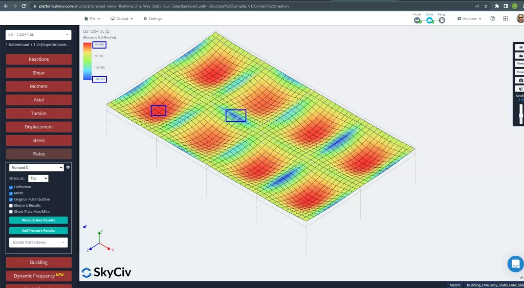
Figuur 26. Platenmomenten in de X-richting. (Structurele 3D, SkyCiv Cloud-engineering).
Afbeeldingen 27 en 28 bestaan uit het buigmoment in elke hoofdrichting. Het nemen van de momentverdeling en waarden, de software, SkyCiv, kan dan het totale staalversterkingsoppervlak verkrijgen.
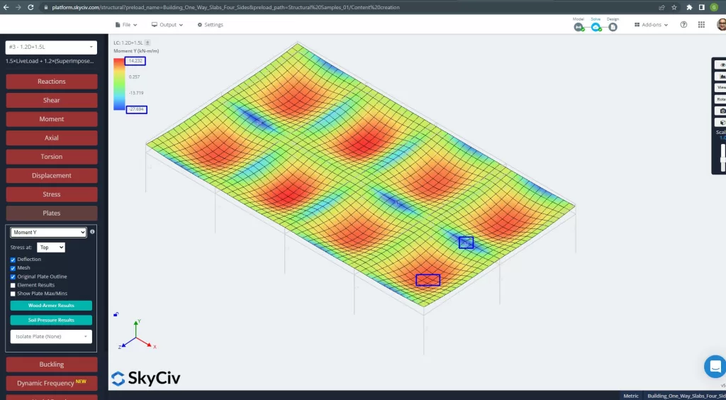
Figuur 27. Platenmomenten in de Y-richting. (Structurele 3D, SkyCiv Cloud-engineering).
Stalen versterkingsgebieden:
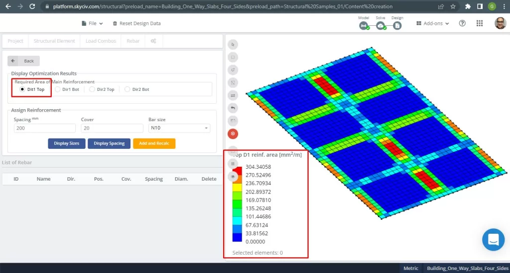
Figuur 28. Versterking van stalen wapening bovenaan in de richting 1. (Structurele 3D, SkyCiv Cloud-engineering).
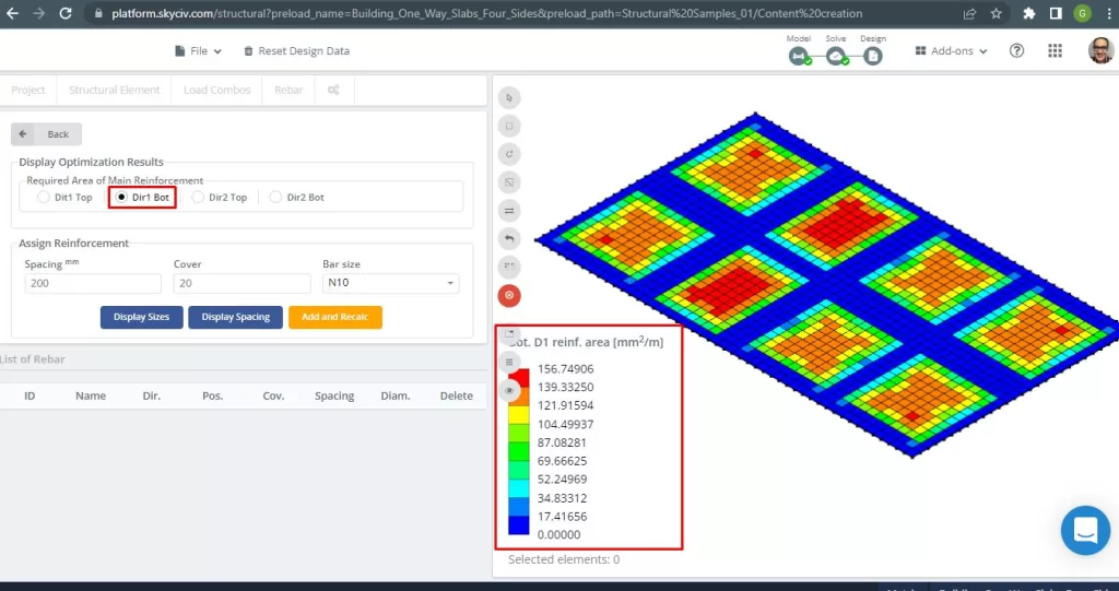
Figuur 29. Versterking van stalen wapening onderaan in de richting 1. (Structurele 3D, SkyCiv Cloud-engineering).
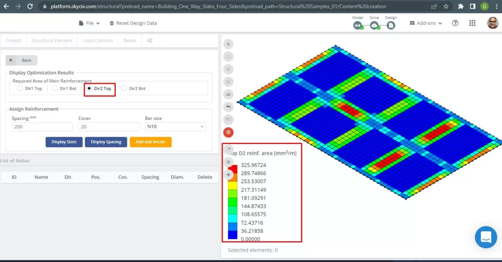
Figuur 30. Versterking van stalen wapening bovenaan in de richting 2. (Structurele 3D, SkyCiv Cloud-engineering).
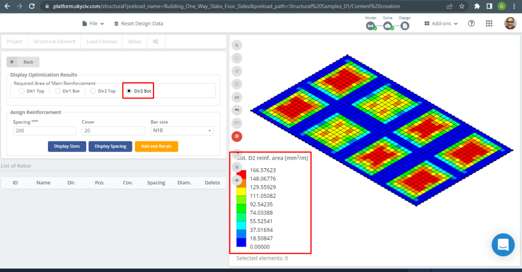
Figuur 31. Versterking van stalen wapening onderaan in de richting 2. (Structurele 3D, SkyCiv Cloud-engineering).
Vergelijking van resultaten
De laatste stap in dit voorbeeld van een eenrichtingsplaatontwerp is het vergelijken van het gebied van de stalen wapening verkregen door S3D-analyse en handmatige berekeningen.
Wapeningsstaal voor X-richting
| Momenten en staalgebied | Exterieur Negatief Links | Exterieur Positief | Exterieur negatief recht | Binnenlands Negatief Links | Interieur Positief | Binnenlands negatief recht |
|---|---|---|---|---|---|---|
| \(EEN_{de opwaartse bodemdruk veroorzaakt bidirectionele buiging met trekspanningen aan het bodemoppervlak, HandCalcs} {mm^2}\) | 334.8214 | 334.8214 | 335.08233 | 334.821 | 334.8214 | 334.8214 |
| \(EEN_{de opwaartse bodemdruk veroorzaakt bidirectionele buiging met trekspanningen aan het bodemoppervlak, S3D} {mm^2}\) | 289.75 | 149.35 | 325.967 | 325.967 | 116.16 | 217.311 |
| \(\Delta_{verschil}\) (%) | 13.461 | 55.39 | 2.720 | 2.644 | 65.307 | 35.0964 |
Wapeningsstaal voor Y-richting
| Momenten en staalgebied | Exterieur Negatief Links | Exterieur Positief | Exterieur negatief recht | Binnenlands Negatief Links | Interieur Positief | Binnenlands negatief recht |
|---|---|---|---|---|---|---|
| \(EEN_{de opwaartse bodemdruk veroorzaakt bidirectionele buiging met trekspanningen aan het bodemoppervlak, HandCalcs} {mm^2}\) | 334.821 | 334.821 | 334.821 | 334.821 | 334.821 | 334.821 |
| \(EEN_{de opwaartse bodemdruk veroorzaakt bidirectionele buiging met trekspanningen aan het bodemoppervlak, S3D} {mm^2}\) | 270.524 | 156.75 | 304.34 | 304.34 | 156.75 | 270.52 |
| \(\Delta_{verschil}\) (%) | 19.203 | 53.184 | 9.104 | 9.104 | 53.184 | 19.204 |
Het verschil is wat groot voor positieve momenten en de reden zou de aanwezigheid zijn van balken met een hoge torsiestijfheid die van invloed zijn op de plaateindige-elementenanalyseresultaten en de berekeningen voor het buigen van wapeningsstaal..
Als je nieuw bent bij SkyCiv, Meld u aan en test de software zelf!
Referenties
- Yew-Chaye Loo & Sanual knuffel Chowdhury , “Gewapend en voorgespannen beton”, 2e editie, Cambridge University Press.
- Bazan Enrique & Meli Piralla, “Seismisch ontwerp van constructies”, 1ed, DUIDELIJK.
- Australische standaard, Betonnen constructies, ALS 3600:2018