Case Study: SkyCiv and Python Programming for Structural Analysis of Planar Frames

Have you ever asked yourself how structural software essentially works? Just keep reading, and you will find how we can use the SkyCiv platform and Python programming through an example developed in a classroom of Structural Analysis.

A quick review of structural analysis

We often use software available to solve a structural analysis, which results in forces, displacement, stresses, etc. In simple terms, the problem drops into the following form:F=K∙d

F=K∙d

$F = K bullet d$

Where:

• F is the vector forces
• K is the structure stiffness
• d is the displacement field

The main goal is to convert a continuous structure into discrete “pieces” of an assembly and analyze it, obtaining forces and displacements. A general path has to be followed:

• Preprocess: the first step in structural analysis, where we get the structure data, geometry, material properties, and loads and finalize when the global stiffness matrix is constructed.
• Process: where we solve the previous expression, F=K∙d F=K∙d$F=Kbullet d$. Some methods generally accepted to solve the linear equations system is Gauss-Jordan, Gaussian elimination, etc.
• Postprocess: the final part to display the results in terms of forces and stress, if necessary.

Planar frame example

The case example consists of a regular planar frame (Figure 1).

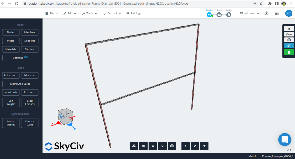
Figure 1. Structural 2D Frame Example

The element’s properties for columns, beams, and materials are:

Concrete properties:

• Material strength, f′c=20MPa     f′c=20MPa$f'c = 20 MPa$
• Young’s Modulus, E=17000MPa E=17000MPa$E = 17000 MPa$

Python programming and SkyCiv Modelling

Now is the time to start working in parallel with modeling in Python and SkyCiv. Figure 2 shows the input data (nodes, elements, degrees of freedom, local axis orientation) for the code developed in Python. You can check the file yourself and run the example through this link.

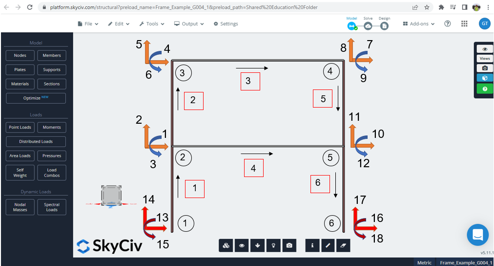
Figure 2. Local stiffness matrix function

The Python file uses a functional programming paradigm because it is easy to explain and develop in the classroom. This consists of dividing and conquering, modularizing the code construction and its methods.

When coding the method, the most important is to define the mathematical formulation to apply.  We will use the Euler Bernoulli Beam:

In summary, the steps required to run the analysis using Python programming are as follows (We reproduce some parts of the Python script):

• Define nodes and their coordinates (xi, yi )

• Determine the global stiffness matrix for each element (kg)

• Assembly of the global structure stiffness matrix (Sg )

• Determine the global load vector for each element and assembly it into the general structure load vector (P, Pf)

• Solve the general equation for the field displacement ({P – P_f} = [S]{d})

• Obtain the global and local forces for each element (Fi, Qi)

The differences in values (Python Script and SkyCiv S3D) are minor, with approximately 2.90% as the mean.

2. Axial forces

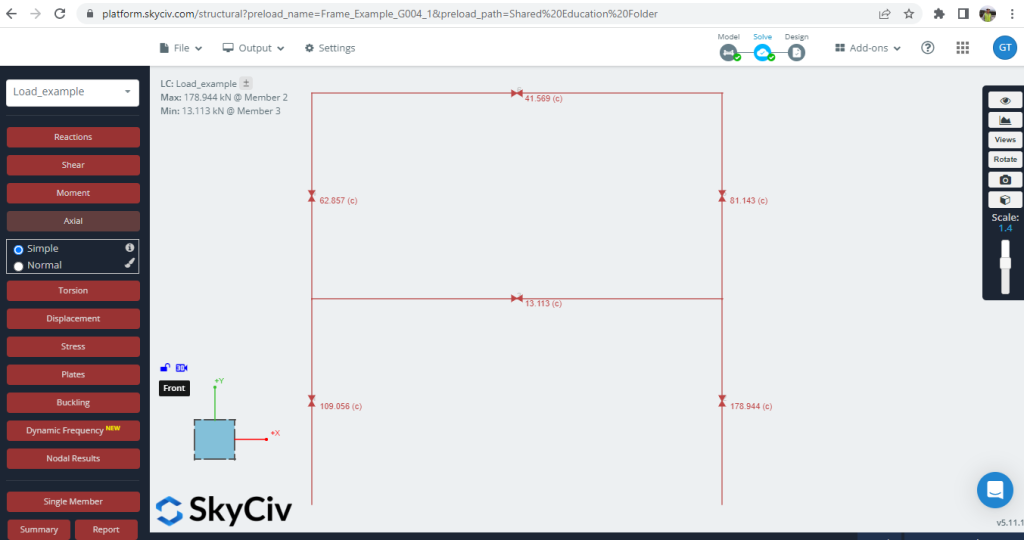
Figure 5. Axial forces developed into the frame

The differences in values (Python Script and SkyCiv S3D) are minor, with approximately 2.65 % as the mean.

3. Shear forces

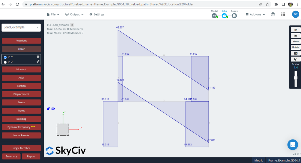
Figure 6. Shear forces developed into the frame

4. Bending moments

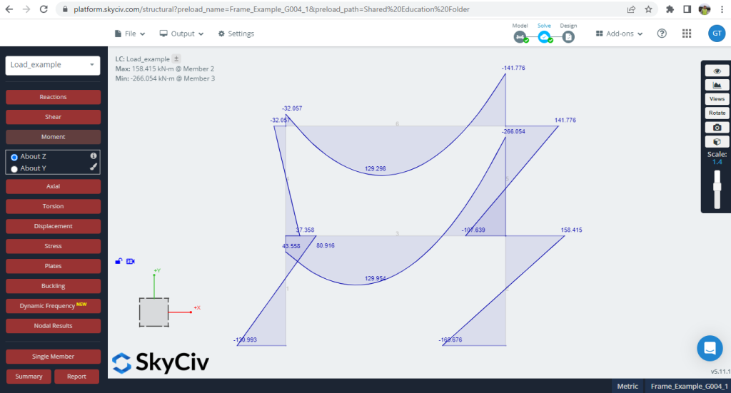
Figure 7. Moments developed into the frame