Supercharging the Design Process with SkyCiv for Grasshopper

Engineers love efficiency, there is no doubt about that. When we notice repetition, we typically seek a method for automation. As one of the leading providers of engineering automation, we have been watching the desire to create increasingly efficient processes snowball over the years.

One of the most popular tools in the parametric design world is Grasshopper 🦗 … a Rhino3d 🦏 plugin – yep, animal names seem to be a common theme around here! We see this as an extremely powerful model generative tool, which is why we have a fully functional integration with Grasshopper via the SkyCiv – Grasshopper Plugin.

Rhino is a powerful 3D modeling software that provides a well-documented API for all of its modeling entities. Grasshopper is a visual programming language, meaning, you can drop various “components” into the viewport that have a specific task. You then feed the output from one component into another component. In programming terms, Grasshopper components are functions. There are hundreds of built-in components to get you started but what’s better is that you can create your own using Python, C#, VB, or even more simply, a combination of existing components.

So buckle up and let’s create the Structural Engineers’ equivalent of the “Hello World” script; a portal frame shed!

We will break this into two sections:

1. How to create the geometry of a portal frame shed using Grasshopper;
2. Converting the geometry to a SkyCiv structure for analysis.

By the end of stage 1, you will have a parametric script that generates the basic geometry of a portal frame shed as seen below. 

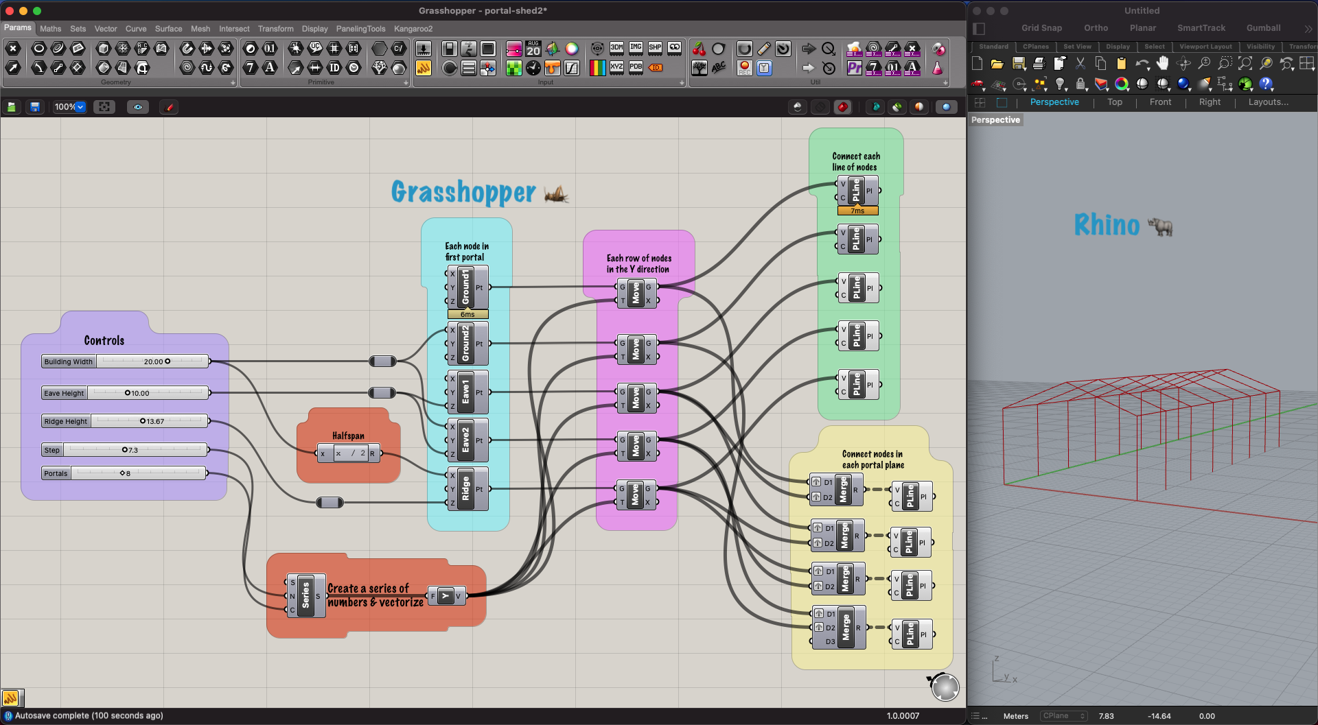
Figure 1. A simple Grasshopper script to create the geometry of a Portal Frame Shed.

Tutorial

First things first, head over to the Rhino3d download page and download and install the right package for your computer. At the time of writing, we are using Rhino7.

Now open Rhino and create a new project from the “standard templates” section. Likely either Large Objects – feet or Large Objects – Meters, I will be working with meters however this won’t make any difference during the first stage. Now you should have a viewport divided into 4 different views, if you’d prefer a single view, just click perspective. 

Next, launch Grasshopper, it can be found in the standard menu or by typing “Grasshopper” into the command field.

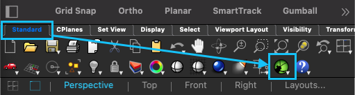
Figure 2. Launching grasshopper.

Now we can start adding components to the Grasshopper view. This can be done in a few ways, if you know the name of the component, just tap the spacebar or double click anywhere in the Grasshopper view, type in the name, and hit enter. Alternatively, you can click a component in the menu and then click where you want to place it.

Let’s go on a quick tangent to get familiar with the UI.

Start by adding a number slider: spacebar → “number slider” → enter. This will drop a slider into the view with a lower bound of “0”, an upper bound of “1”, and a step size of “0.001”. You can double click the slider to adjust these parameters but there is a faster way! Spacebar → “0..30.00” → enter. This will create a slider with a lower bound of “0.00”, an upper bound of “30.00”, and a step size of “0.01” (because we used “30.00”). 0.00..30 would achieve the same result.

Another good tool is the Panel tool, this is essentially a sticky note that will display the output value of a component. The shortcut for the panel is a single double-quote followed by its contents. So now tap the spacebar → “ → enter and you will have a panel. Drag the output node of your number slider and drop it on the input node of the panel. Now you will see the value of the slider update in the panel as you slide it!

Next, add the Construct Point component. You will see a point appear in the Rhino window at the coordinate system origin. Connect the slider value to one or more of the point coordinates (either directly or through the panel) and you will be able to move the point with the slider, awesome right?  You can disconnect wires by holding Ctrl (or Cmd) and redrawing them. By clicking a component in Grasshopper such as construct point, it will appear green in Rhino. 

Try connecting two points with a line; hint: have a look in the Curve → Primitive menu. Without the line, this is something like what you should be experimenting with now.

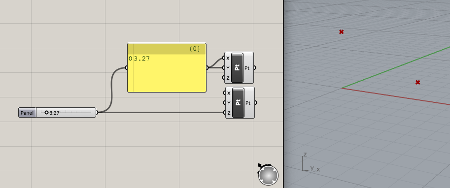
Figure 4. Plotting points in Rhino3d from Grasshopper.

Now that you’ve familiarized yourself with the basics, let start creating the shed! Referencing figure 1, we will work our way through each group defined by the colored containers, starting with the left-most violet-colored group.

Violet

This is usually where I would start with a script, it’s similar to your variable declarations at the top of your code. Have a think about what parameter you would like to be used and need, to define the geometry. Go ahead and create your sliders,  practice the shortcut!

1. Building Width – the distance from column to column of the portals.
2. Eave Height – The height of the columns.
3. Ridge Height – The height from the ground to the ridge.
4. Step – The distance between each portal.
5. Portals – The number of portals, note this is an integer: space → 1..20 → enter.

Note: If you’d like to organize the script (highly recommended), you can drag and select multiple items, then right-click in empty space and group the items. The component showing “Controls” is called Scribble. You can then right-click the green group and customize it as you like.

Orange

In the orange groups, we are calculating other variables that we will need based on the input.  This is also a good time to introduce the Relay. Double-click a wire to add a relay, they are helpful to keep everything organized and allow branching off. Double-click the relay again to remove it.

The first component is the Expression component which allows us to plug some variables in, write a mathematical expression and pass the result (R) out. If you zoom in close, a ➕ and ➖ button will appear to add or remove more variables to the component. This is the case for many other components too. Double-click on the component and type x/2 into the expression field. Now we have the half span which will help us plot the ridgeline.

In the second orange group, we are using the series component to create a series of numbers which will provide us a Y coordinate for each portal. The inputs for the series component are “start” (S), “step size” (N), and “count” (C). If we don’t provide S with an input, it will default to 0. Confirm this by waving the mouse over the S. Connect your step slider to N and your Portals slider to C. Either wave over the output of the series or just plug it into the trusty panel to see the output values. Now we have a series of Y positions but… Grasshopper is interpreting these values simply as numbers, not Y coordinates. Convert this array of numbers to Y vectors by sending them into a Unit Y component, spacebar → Y → enter. Now have a look at the output and you will see the numbers have been processed into coordinates. Note that the output wire of the series component is thicker. This indicates that there are multiple values in the output (an array) not just a single value.

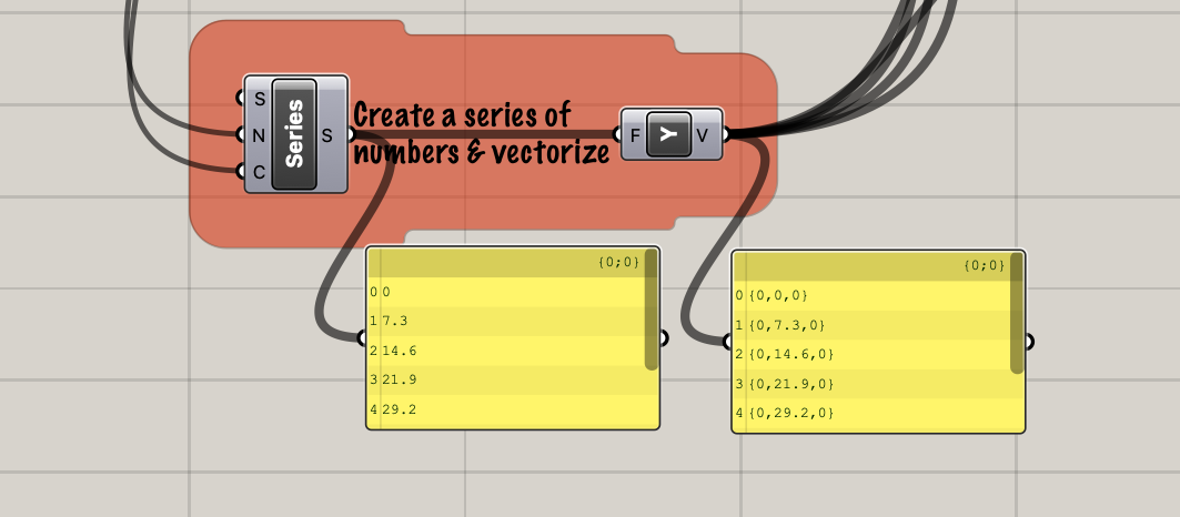
Figure 5. Creating a series of coordinates.

Blue

In the blue group, we are plotting the points that make up the first portal; five points per portal. Add five of the Construct Point components that we used earlier and try connecting correct inputs. Use figure 1 for a reference if you get stuck. You can right-click the component to give it a label. You might need to turn off Draw Icons to display the name of the component rather than the icon. This can be found in the display menu (the window display menu, not the Grasshopper display menu!). 

Now you should be able to use the sliders to adjust the portal nodes. 

Pink

By now you might realize, there are millions of ways to reach our goal and many that might be more efficient. The path we are taking, I decided was a good option as it will keep the various geometry elements in separate components and introduce a few different tools so we don’t end up with one component that outputs a big, jumbled mess of items.

Onto the Move component. This component takes geometry (G) and motion (T). It is smart enough to know that if you provide multiple motion values, it should iterate them and apply each of them to the geometry parameter. Hook up each of our portal points accompanied by our series of Y vectors and you will see multiple portals in a line. Adjust your Step and Portal slider to see the change.

Notice how if you click one of your point components in the blue zone, you will see one point in Rhino, then click the Move component that it feeds to and you will see a green point in the same position plus the others. This is important! Each component is not adjusting the previous component, rather, it is creating a duplicate, then adjusting that duplicate. Now we have our rows of points, drag and highlight all the components of the blue group, right-click in empty space, and select preview off, we don’t need to see these in Rhino anymore. These options can also be found in the round menu when you middle-click. If you’re using a magic mouse you can get this menu with option+spacebar. 

Green

In the green section, we connect the ridge and eave points with a PolyLine. This will take an ordered list of vertices (V) and plot a line through them. The other parameter (C) indicates whether the line should close, i.e connect the final point to the first. You might connect a Boolean Toggle into this however we won’t. The two lines connecting the column bases are likely redundant so you can leave them out. 

Yellow

In this section, we are creating the column and rafter lines. There is a little bit of complex magic used here so don’t be too hard on yourself if you don’t understand it the first time around. 

Starting from the end, the PolyLine component needs an ordered list of points to connect. For the first column, we have a row of points along the ground and a row of points along the eave. We need to manipulate this data into groups of two points, each column’s start-point, and end-point. We can use the Merge component to bring these two rows of points together, so feed the two rows into the Merge component and then into the PolyLine component, you will notice a Z shape is created. This is because naturally, the Merge component will just combine the two lists together into one,  larger list. Wave over the Merge input and you will see something like “Data 1 as Tree”, this means we need to covert our array of points into a tree before running the merge. Right-click both D1 and D2 on the Merge component and click “Graft” for each, a ⬆️ will appear next to each input. Now the columns look ok…but why? Plug the Merge output into a panel and then look at the difference as you flick graft on and off. 

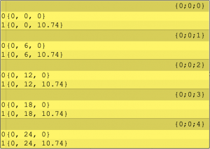
Figure 6. Merged tree data.

Without diving too deep, “graft” will take a list of items and put them into their own groups,  each group could then contain a list. So when we try to merge two trees, each of which contains the same amount of groups, it will merge groups with the same index.

Go ahead and connect the column and rafters. Voilà, hello shed! 

Closing thoughts

We’ve now seen how user-friendly and extraordinarily powerful Grasshopper is. With a bit of practice, you will be able to create a script like this in half an hour. Imagine the possibilities if you allocate some decent resources. Look out for Part 2 where we will use the SkyCiv Grasshopper plugin to run a Structural Analysis on the shed.